4Classical Machine Learning 4.4Model Ensembles
4.4.2XGBoost
Gradient boosting of decision trees: fitting residuals and gradients, the regularised objective of XGBoost, early stopping and tuning, and scikit-learn's histogram-based gradient boosting.
Boosting builds a model the way a draft is revised: each round looks at what is still wrong and adds a small correction, in this case a small decision tree aimed at the remaining errors. After many rounds, these small corrections add up to a very accurate model.
On tables of features, gradient-boosted trees are among the most accurate models available, and they are a common choice whenever the best possible score matters. They also work well on features taken from a pretrained network, which is why XGBoost appears next to logistic regression in the hints for Ghost of the Machine (IOAI 2026).
The price of that accuracy is care. Boosting has more hyperparameters than a random forest and overfits more easily, so it needs a good validation set and early stopping. This module explains how boosting works, what XGBoost adds to it, and how to train and tune it without overfitting.
XGBoost is a library for gradient boosting of decision trees. A boosted model, like a random forest, is an ensemble of trees. A forest grows its trees independently and averages them to reduce variance, whereas boosting grows small trees one after another, each fitted to the errors that the previous trees still make. The IOAI 2026 Technical Appendix lists xgboost among the core machine learning libraries of the contest environment, together with lightgbm and catboost, two other gradient-boosting libraries. This module assumes Decision Trees.
Boosting
In gradient-boosted trees, each is a small regression tree, even in classification, where is a real-valued score such as the log-odds of logistic regression.
| Random forest | Gradient boosting | |
|---|---|---|
| Trees | Independent, each on a bootstrap sample | Sequential, each fitted to the current errors |
| Depth | Unlimited by default in scikit-learn | At most 6 by default in XGBoost |
| Combination | Average | Sum, scaled by |
| Mainly reduces | Variance | Bias |
| Adding trees | The score levels off | The model can overfit |
Gradient boosting for regression
With squared error, each round fits a regression tree to the residuals , the part of each label that the current model does not yet explain. The worked example below uses six samples with one feature, decision stumps (trees of depth 1) and . The table follows the predictions through two rounds.
| Sample 1 | 2 | 3 | 4 | 5 | 6 | MSE | |
|---|---|---|---|---|---|---|---|
| Feature | 1 | 2 | 3 | 4 | 5 | 6 | |
| Label | 1 | 1 | 4 | 4 | 4 | 10 | |
| Start | 4 | 4 | 4 | 4 | 4 | 4 | 9 |
| Residual | −3 | −3 | 0 | 0 | 0 | 6 | |
| Stump 1, split at | −1.2 | −1.2 | −1.2 | −1.2 | −1.2 | 6 | |
| stump 1 | 3.4 | 3.4 | 3.4 | 3.4 | 3.4 | 7 | 3.6 |
| Residual | −2.4 | −2.4 | 0.6 | 0.6 | 0.6 | 3 | |
| Stump 2, split at | −2.4 | −2.4 | 1.2 | 1.2 | 1.2 | 1.2 | |
| stump 2 | 2.2 | 2.2 | 4 | 4 | 4 | 7.6 | 1.44 |
- Start. The mean label, 4, minimises squared error, as shown for regression trees.
- Each stump predicts the mean residual on each side of its split. Of the thresholds 1.5 to 5.5, stump 1's split at leaves the smallest squared error about the two leaf means (10.8).
- Stump 2 splits elsewhere because round 1 already removed half of the error of sample 6: each round fits what the current sum still gets wrong.
import numpy as np
from sklearn.tree import DecisionTreeRegressor

X = np.array([[1], [2], [3], [4], [5], [6]], dtype=float)
y = np.array([1, 1, 4, 4, 4, 10], dtype=float)

F = np.full(len(y), y.mean())     # F_0 = 4 for every sample
for m in range(2):
    stump = DecisionTreeRegressor(max_depth=1)
    stump.fit(X, y - F)           # fit the residuals
    F = F + 0.5 * stump.predict(X)
    mse = np.mean((y - F) ** 2)
    print(stump.tree_.threshold[0], F.round(2), round(mse, 2))
# 5.5 [3.4 3.4 3.4 3.4 3.4 7. ] 3.6
# 2.5 [2.2 2.2 4. 4. 4. 7.6] 1.44function gradient_boosting(X, y, n_rounds, learning_rate):
F0 = mean(y) # starting prediction
F = F0 for every sample # current predictions
trees = []
repeat n_rounds times:
residuals = y - F
tree = small regression tree fitted to (X, residuals)
F = F + learning_rate * tree.predict(X) # learning_rate is η
trees.append(tree)
return F0, trees
# prediction for a new sample x:
# F0 + learning_rate * (sum of tree.predict(x) over all trees)The learning rate
The learning rate scales every tree, as it scales every step of gradient descent; in boosting, this is called shrinkage. With , the first stump would have fitted sample 6 exactly in a single round. A smaller corrects only part of the remaining error in each round, so more rounds are needed, and the scikit-learn User Guide notes that small learning rates empirically favour a lower test error.
Gradient boosting with any loss
For , the derivative with respect to the prediction is . The residual is therefore the negative gradient, and fitting a tree to the residuals is a step of gradient descent on the predictions . The same step applies to any differentiable loss.
Loss Functions describes the losses; their pseudo-residuals are:
| Loss | Pseudo-residual | |
|---|---|---|
| Squared error | ||
| Absolute error | ||
| Log loss, with |
Classification. For two classes, is the log-odds of class 1, and with the sigmoid function. The derivative of log loss with respect to the log-odds is , as derived for logistic regression, so the pseudo-residual is . For labels 1, 1, 1 and 0, the initial score is , every sample has , and the pseudo-residuals are , , and . For classes, XGBoost fits one tree per class in every round and combines the scores with the softmax function; on the Wine dataset, 50 rounds give 150 trees.
For other losses, the mean pseudo-residual of a leaf is not the best leaf value; XGBoost computes leaf values from the second derivative of the loss, as the next section shows.
The XGBoost objective
XGBoost (Chen and Guestrin, 2016) extends gradient boosting in two ways: it penalises the complexity of each tree, and it uses the second derivative of the loss as well as the first.
The regularised objective
A tree with leaves sends each sample to a leaf and outputs that leaf's weight . In round , XGBoost looks for the tree that minimises
The penalty charges for every leaf and for large weights, as Ridge regression does for coefficients. The learning rate is applied afterwards, to the weights of the finished tree.
Each sample's loss is replaced by its second-order Taylor approximation around the current prediction, , where and are the first and second derivatives of the loss with respect to the prediction at . For squared error, and , so the approximation is exact; for log loss, and .
Leaf weights and split gain
With and the sums of and over the samples in leaf , and terms that do not depend on the tree dropped, the objective separates into one parabola per leaf:
Its minimum gives the optimal weight of each leaf and the best objective for the tree structure:
Splitting a leaf into a left child and a right child therefore lowers the objective by the gain
At each node, XGBoost chooses the split with the largest gain. A split with negative gain saves less than the cost of its extra leaf, so acts as the minimum loss reduction required to split.
In the worked example, gives and . With and , the two best splits are:
| Split | Gain | ||||||
|---|---|---|---|---|---|---|---|
| 6 | 2 | −6 | 4 | −2 | 1.2 | 9.6 | |
| 6 | 5 | −6 | 1 | −1 | 3 | 12 |
The split at 5.5 still wins, with weights and instead of the mean residuals and : the penalty halves the weight of the one-sample leaf and barely changes the five-sample leaf. With , is exactly the mean residual, so plain gradient boosting is the special case .
Checking the formulas
With reg_lambda=0, XGBoost reproduces the worked example. XGBoost 3.4.1 estimates the initial prediction from the labels and stores it in intercept_.
from xgboost import XGBRegressor

xgb_reg = XGBRegressor(n_estimators=2, learning_rate=0.5, max_depth=1,
                       reg_lambda=0.0)
xgb_reg.fit(X, y)
print(xgb_reg.intercept_, xgb_reg.predict(X))
# [4.] [2.2 2.2 4.  4.  4.  7.6]
For log loss, a one-tree model on the breast cancer dataset (label 1 means benign) with base_score=0.5 starts every sample at , so and .
from sklearn.datasets import load_breast_cancer
from xgboost import XGBClassifier

X_bc, y_bc = load_breast_cancer(return_X_y=True)  # 1 = benign
one_tree = XGBClassifier(n_estimators=1, max_depth=2,
                         learning_rate=0.3, reg_lambda=1.0,
                         base_score=0.5)
one_tree.fit(X_bc, y_bc)

p = 0.5                              # initial probability of class 1
g = p - y_bc                         # first derivatives g_i
h = np.full(len(y_bc), p * (1 - p))  # second derivatives h_i
leaf = one_tree.apply(X_bc)          # leaf reached by each sample
nodes = one_tree.get_booster().trees_to_dataframe()
for j in np.unique(leaf):
    G, H = g[leaf == j].sum(), h[leaf == j].sum()
    w_star = -G / (H + 1.0)
    stored = nodes.loc[nodes["Node"] == j, "Gain"].item()
    print(int(j), G, H, round(0.3 * w_star, 4), round(stored, 4))
# 3 -165.0 91.0 0.538 0.538
# 4 9.0 5.5 -0.4154 -0.4154
# 5 1.5 4.75 -0.0783 -0.0783
# 6 82.0 41.0 -0.5857 -0.5857
In trees_to_dataframe(), the Gain column of a leaf holds its output , and all four leaves agree with the formula. For a split, the column holds twice the gain defined above.
Histogram-based split finding
Instead of sorting each feature at every node, as CART does, XGBoost's default tree_method="auto" (the same as "hist") divides each feature into at most max_bin = 256 bins before training, sums and per bin at each node, and evaluates the gain only at bin boundaries. The scikit-learn User Guide gives the cost of splitting a node as with histograms, against with sorting.
Training XGBoost in Python
XGBClassifier and XGBRegressor follow the scikit-learn estimator interface, and, like all tree models, they need no feature scaling.
import xgboost
from sklearn.metrics import accuracy_score, log_loss
from sklearn.model_selection import train_test_split

print(xgboost.__version__)  # 3.4.1
X, y = load_breast_cancer(return_X_y=True, as_frame=True)
X_train, X_test, y_train, y_test = train_test_split(
    X, y, test_size=0.25, stratify=y, random_state=0
)
model = XGBClassifier(n_estimators=200, learning_rate=0.1,
                      max_depth=3, random_state=0)
model.fit(X_train, y_train)

score = model.predict(X_test, output_margin=True)  # F(x), log-odds
proba = model.predict_proba(X_test)[:, 1]          # P(benign)
print(score[:3].round(2))
# [ 7.98 -8.05 -7.97]
print([round(float(v), 4) for v in proba[:3]])
# [0.9997, 0.0003, 0.0003]
print(np.allclose(proba, 1 / (1 + np.exp(-score))))  # True
print(accuracy_score(y_test, model.predict(X_test)))
# 0.951048951048951
print(round(log_loss(y_test, proba), 4))  # 0.1635
For two classes, the objective is binary:logistic: predict with output_margin=True returns the score , and the second column of predict_proba is . XGBClassifier requires the classes to be numbered ; labels and raise a ValueError.
Missing values
XGBoost accepts NaN in the features without imputation. As in scikit-learn's trees, each split stores a default direction for missing values, chosen during training by the larger gain (section 3.4 of the XGBoost paper).
rng = np.random.default_rng(0)
X_train_nan = X_train.mask(rng.random(X_train.shape) < 0.2)
X_test_nan = X_test.mask(rng.random(X_test.shape) < 0.2)

model_nan = XGBClassifier(n_estimators=200, learning_rate=0.1,
                          max_depth=3, random_state=0)
model_nan.fit(X_train_nan, y_train)  # no imputation
print(accuracy_score(y_test, model_nan.predict(X_test_nan)))
# 0.9370629370629371
nodes = model_nan.get_booster().trees_to_dataframe()
print(nodes.loc[:2, ["Feature", "Split", "Yes", "No", "Missing"]])
#                 Feature   Split  Yes   No Missing
# 0          worst radius   16.84  0-1  0-2     0-1
# 1  worst concave points  0.1424  0-3  0-4     0-3
# 2       worst concavity   0.221  0-5  0-6     0-6
A sample goes to the Yes child when its value is below Split, and a missing value follows Missing. With 20% of the values missing, 134 of the 143 test tumours are still classified correctly. The argument missing marks another value, such as −999, as missing, and XGBoost 3.4.1 also accepts pandas columns of dtype category directly.
Early stopping
A boosted model can overfit as rounds are added, so the number of rounds is chosen on a validation set. In the synthetic problem below, flip_y=0.1 assigns 10% of the labels at random, and the 6,000 samples are split into 3,600 for training, 1,200 for validation and 1,200 for testing.
from sklearn.datasets import make_classification

X_s, y_s = make_classification(n_samples=6000, n_features=20,
                               n_informative=6, flip_y=0.1,
                               random_state=0)
X_rest, X_te, y_rest, y_te = train_test_split(
    X_s, y_s, test_size=0.2, stratify=y_s, random_state=0)
X_tr, X_val, y_tr, y_val = train_test_split(
    X_rest, y_rest, test_size=0.25, stratify=y_rest, random_state=0)

es = XGBClassifier(n_estimators=3000, learning_rate=0.1,
                   early_stopping_rounds=50, eval_metric="logloss",
                   random_state=0)
es.fit(X_tr, y_tr, eval_set=[(X_tr, y_tr), (X_val, y_val)],
       verbose=False)
print(es.best_iteration)                      # 65
print(es.get_booster().num_boosted_rounds())  # 116
history = es.evals_result()
val_loss = history["validation_1"]["logloss"]
print(round(val_loss[es.best_iteration], 4))  # 0.3329
print(es.score(X_te, y_te)) # 0.8641666666666666| Round | 1 | 10 | 25 | 50 | 66 | 100 | 116 |
|---|---|---|---|---|---|---|---|
| Training log loss | 0.6334 | 0.3673 | 0.2344 | 0.1654 | 0.1408 | 0.1040 | 0.0895 |
| Validation log loss | 0.6418 | 0.4330 | 0.3549 | 0.3373 | 0.3329 | 0.3365 | 0.3379 |
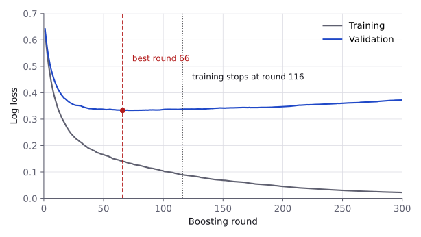
The validation loss is lowest at round 66 and then rises, while the training loss keeps falling.
- Arguments.
early_stopping_roundsis a constructor argument: in XGBoost 3.4.1,fitrejects it with aTypeError, and early stopping withouteval_setraises aValueError. The last entry ofeval_setdecides when to stop. - The best round.
best_iterationcounts from 0.predict,predict_probaandscoreuse only the trees up to it, although all 116 are stored. - Separate data. The validation score that chose the round is optimistic, so the test set must stay unused. When the model is refitted on all labelled data for the submission,
n_estimators=best_iteration + 1fixes the number of rounds.
Hyperparameters
XGBClassifier().get_params() shows None for most hyperparameters, meaning that XGBoost's own default applies. The defaults below, from the XGBoost Parameters documentation, match the configuration that get_booster().save_config() reports for a model trained with version 3.4.1.
| Parameter | Default | Meaning |
|---|---|---|
n_estimators |
100 | Number of boosting rounds |
learning_rate |
0.3 | (alias eta) |
max_depth |
6 | Maximum depth of each tree |
min_child_weight |
1 | Minimum in a child; for squared error, a number of samples |
gamma |
0 | , the minimum gain of a split |
reg_lambda |
1 | , the L2 penalty on leaf weights |
reg_alpha |
0 | L1 penalty on leaf weights |
subsample |
1 | Fraction of training samples drawn in each round |
colsample_bytree |
1 | Fraction of features drawn for each tree |
scale_pos_weight |
1 | Weight of the positive class in imbalanced binary problems |
random_state |
0 | Seed for the random sampling |
The learning rate and the number of rounds are chosen together. On the split of the previous section:
for lr in [0.3, 0.1, 0.03]:
    m = XGBClassifier(n_estimators=3000, learning_rate=lr,
                      early_stopping_rounds=50,
                      eval_metric="logloss", random_state=0)
    m.fit(X_tr, y_tr, eval_set=[(X_val, y_val)], verbose=False)
    print(lr, m.best_iteration + 1, round(m.best_score, 4),
          round(m.score(X_te, y_te), 3))
# 0.3 18 0.3377 0.861
# 0.1 66 0.3329 0.864
# 0.03 240 0.3344 0.869
Dividing the learning rate by about 3 multiplies the best number of rounds by about 3.6, while the validation losses differ by less than 0.005.
XGBoost's "Notes on Parameter Tuning" separates hyperparameters that control model complexity (max_depth, min_child_weight, gamma) from those that add randomness (subsample, colsample_bytree). A practical order is to fix learning_rate=0.1 and set n_estimators by early stopping; to tune the complexity group, then the randomness group, then reg_lambda and reg_alpha if the model still overfits; and finally to lower the learning rate if time allows. Hyperparameter Tuning describes the search methods.
Gradient boosting in scikit-learn
Scikit-learn's HistGradientBoostingClassifier and HistGradientBoostingRegressor also bin the features, and they accept NaN values and categorical features directly. Their defaults in scikit-learn 1.9.1 are:
| Parameter | Default | Closest XGBoost parameter |
|---|---|---|
max_iter |
100 | n_estimators (100) |
learning_rate |
0.1 | learning_rate (0.3) |
max_leaf_nodes |
31 | max_leaves (0, no limit) |
max_depth |
None |
max_depth (6) |
min_samples_leaf |
20 | min_child_weight (1) |
l2_regularization |
0.0 | reg_lambda (1) |
max_bins |
255 | max_bin (256) |
early_stopping |
"auto" |
early_stopping_rounds (off) |
With early_stopping="auto", early stopping is switched on when the training set has more than 10,000 samples, or when X_val and y_val are passed to fit. The estimator then holds out validation_fraction=0.1 of the training data and stops when the loss has not improved for n_iter_no_change=10 iterations.
from sklearn.ensemble import HistGradientBoostingClassifier

for n in [10_000, 10_001]:
    X_n, y_n = make_classification(n_samples=n, random_state=0)
    hgb = HistGradientBoostingClassifier(random_state=0).fit(X_n, y_n)
    print(n, hgb.do_early_stopping_, hgb.n_iter_)
# 10000 False 100
# 10001 True 79
Pandas columns of dtype category are treated as categorical by default (categorical_features="from_dtype"), while a column of strings raises ValueError: could not convert string to float.
import pandas as pd

rng = np.random.default_rng(0)
size = rng.normal(size=2000)
colour = rng.choice(["red", "green", "blue"], 2000)
df = pd.DataFrame({"size": size, "colour": pd.Categorical(colour)})
label = ((df["colour"] == "green") ^ (df["size"] > 0)).astype(int)
df.loc[rng.choice(2000, 200, replace=False), "size"] = np.nan

hgb = HistGradientBoostingClassifier(random_state=0).fit(df, label)
print(hgb.is_categorical_)             # [False  True]
print(round(hgb.score(df, label), 3))  # 0.952
The comparison below fits three models with default hyperparameters to 15,000 training samples with 40 features and scores them on 5,000 test samples.
import time
from sklearn.ensemble import RandomForestClassifier

X_c, y_c = make_classification(n_samples=20000, n_features=40,
                               n_informative=15, n_redundant=5,
                               flip_y=0.03, random_state=0)
Xc_train, Xc_test, yc_train, yc_test = train_test_split(
    X_c, y_c, test_size=0.25, stratify=y_c, random_state=0)
candidates = {
    "random forest": RandomForestClassifier(n_jobs=-1, random_state=0),
    "HistGradientBoosting": HistGradientBoostingClassifier(
        random_state=0),
    "XGBoost": XGBClassifier(random_state=0),
}
for name, est in candidates.items():
    start = time.perf_counter()
    est.fit(Xc_train, yc_train)
    seconds = time.perf_counter() - start
    acc = est.score(Xc_test, yc_test)
print(f"{name:21} {acc:.4f} {seconds:.2f} s")| Model | Test accuracy | Fit time |
|---|---|---|
Random forest, n_jobs=-1 |
0.9434 | 0.76–0.92 s |
HistGradientBoostingClassifier |
0.9424 | 0.94–1.53 s |
XGBClassifier |
0.9520 | 0.30–0.40 s |
XGBoost is the most accurate and the fastest here, but such rankings depend on the data and must be measured for each task. Both boosting models use all CPU threads by default; the forest does so only with n_jobs=-1.
Gradient boosting in olympiad tasks
- Tables of features. Gradient-boosted trees suit tabular data and embeddings from a pretrained network. The official hints for the GAITE Contest version of Ghost of the Machine (IOAI 2026), quoted in Logistic Regression, name XGBoost as one classifier for sentence embeddings, and warn that embedding all 35,000 training sentences takes about 15 minutes on a CPU, while the whole run is limited to 10 minutes.
- Task rules. In Lost in Hyperspace (IOAI 2024), supervised models, with boosting trees named explicitly, could not be used as feature extractors.
- Time limits. Training time grows with the number of rounds and the depth of the trees, so the fit time should be measured. The parameter
device="cuda"trains on a GPU. - Determinism. With a fixed
random_state, repeated fits give identical predictions, even with row and column subsampling; the XGBoost FAQ notes that multi-threading and floating-point summation order can still cause small differences between runs. - Versions. Defaults and accepted arguments change between releases, so
xgboost.__version__should match the documentation consulted. The official IOAI 2025 environment pinnedxgboost3.0.2,lightgbm4.6.0 andcatboost1.2.8 in itsrequirements.txt; for 2026, exact versions are published before the contest.
Resources
| Source | Title | Why read it |
|---|---|---|
| XGBoost | Introduction to Boosted Trees | “Additive Training”, “The Structure Score” and “Learn the tree structure” derive the second-order objective, the optimal leaf weights and the split gain in the notation of this module. |
| XGBoost | XGBoost Parameters | Every parameter with its default. “Parameters for Tree Booster” covers eta, gamma, max_depth, min_child_weight, subsample, lambda and alpha. |
| XGBoost | Notes on Parameter Tuning | “Control Overfitting” separates the parameters that limit model complexity from those that add randomness. |
| XGBoost | Using the Scikit-Learn Estimator Interface | “Early Stopping” shows early_stopping_rounds and eval_set with XGBClassifier. |
| scikit-learn | User Guide: Gradient-boosted trees | “Histogram-Based Gradient Boosting” describes HistGradientBoostingClassifier and HistGradientBoostingRegressor, including their support for missing values and categorical features. |
| Google for Developers | Decision Forests course: Gradient boosted decision trees | A short page on fitting each weak model to the errors of the current model, with a section on shrinkage. Its code uses TensorFlow Decision Forests, not XGBoost. |
| StatQuest | Gradient Boost Part 1 (of 4): Regression Main Ideas | The main ideas of gradient boosting for predicting a continuous value, built up one step at a time. |
| StatQuest | XGBoost Part 1 (of 4): Regression | The regression trees that XGBoost builds, explained step by step. It assumes the video on gradient boosting above. |
| Chen and Guestrin | XGBoost: A Scalable Tree Boosting System (2016) | The original paper. Section 2 derives the regularised objective and gradient tree boosting; section 3.4, “Sparsity-aware Split Finding”, describes how missing values are handled. |
Practice problems
| Solved | Source | Problem | Difficulty | Tags |
|---|---|---|---|---|
| IOAI 2026 | Ghost of the Machine | Hard | nlp, embeddings | |
| Kaggle | House Prices - Advanced Regression Techniques | Medium | tabular, regression |