4Classical Machine Learning 4.3Classical Machine Learning Models
4.3.5K-Means Clustering
An unsupervised method that partitions samples into k clusters, each represented by the mean of its samples, by minimising the sum of squared distances from samples to their cluster means.
So far, every model in this section has learned from labelled examples. Data often comes without labels, however, and labelling it can be slow or expensive. Even then, a useful first question is whether the samples fall into natural groups: customers with similar habits, images with similar colours, or measurements that gather around a few typical values.
Clustering answers that question, and k-means is its simplest and most widely used method. It places a small number of centres in the data, assigns every sample to its nearest centre, and moves the centres until the groups settle. No labels are needed at any point.
In a contest, k-means rarely gives the final answer on its own. It is a tool for exploring data, for building new features, and for making use of many unlabelled samples when only a few are labelled. It also has clear limits: it expects compact, roughly round groups, and this module shows what happens when the groups have other shapes.
Clustering divides samples into groups, called clusters, so that samples in the same cluster are similar and samples in different clusters are not. It uses the features alone, without labels, and is therefore a form of unsupervised learning. K-means represents each cluster by the mean of its samples. It is unrelated to K-NN, a supervised method in which counts neighbours rather than clusters.
The k-means objective
The following six samples serve as a running example. In the notation of Terminology, , and .
| Sample | ||
|---|---|---|
| 1 | 1 | |
| 3 | 1 | |
| 2 | 4 | |
| 6 | 5 | |
| 8 | 5 | |
| 7 | 8 |
The first three samples lie in the lower left of the plane and the last three in the upper right.
For the running example, take and . The centroids are
The squared distance from to is . Those from and to are 2 and 4, and those from , and to are 2, 2 and 4, so .
A centroid is generally not one of the samples. The smallest achievable inertia never increases as grows and is 0 at , so inertia alone cannot choose (see Choosing the number of clusters).
The k-means algorithm
There are ways to assign samples to clusters, far too many to try. The best clustering is instead approximated by Lloyd's algorithm, usually called the k-means algorithm.
function kmeans(X, k):
    centroids = k samples of X, chosen at random
    repeat:
        # assignment step
        for each sample i:
            cluster[i] = index of the centroid nearest to X[i]
        # update step
        for each cluster j:
            centroids[j] = mean of the samples with cluster == j
    until no sample changed cluster
    return cluster, centroids
One iteration by hand
Start the running example from and , a poor start because both lie in the lower-left group. The assignment step compares squared distances:
| Sample | To | To | Cluster |
|---|---|---|---|
| 0 | 10 | 1 | |
| 4 | 10 | 1 | |
| 10 | 0 | 2 | |
| 41 | 17 | 2 | |
| 65 | 37 | 2 | |
| 85 | 41 | 2 |
With the starting centroids, these assignments give . The update step moves each centroid to the mean of its cluster:
which lowers to 31.75. In the second iteration, is at squared distance 9 from and 16.3125 from , so it joins cluster 1, and the update gives , and . In the third iteration no sample moves, and the algorithm stops. Scikit-learn reproduces the run, numbering the clusters from 0:
import numpy as np
from sklearn.cluster import KMeans

X = np.array([[1, 1], [3, 1], [2, 4], [6, 5], [8, 5], [7, 8]])
start = np.array([[1, 1], [2, 4]])     # mu_1 = x_1, mu_2 = x_3

km = KMeans(n_clusters=2, init=start, n_init=1).fit(X)
print(km.labels_)            # [0 0 0 1 1 1]
print(km.cluster_centers_)   # [[2. 2.]
                             #  [7. 6.]]
print(km.inertia_, km.n_iter_)  # 16.0 3
Why the algorithm stops
Neither step can increase the inertia. Moving a sample to its nearest centroid cannot increase its term of , and for fixed assignments is smallest at the mean of cluster , where its derivative with respect to is zero; a regression tree's leaf predicts the mean for the same reason. A sample moves only to a strictly closer centroid, so every change strictly lowers and no clustering recurs. There are finitely many clusterings, so the algorithm stops.
Local minima
The algorithm can stop at a clustering that is not the best. Take the corners , , and of a rectangle and . Started from and , the algorithm forms the left and right pairs, with . Started from and , it forms the bottom and top pairs, with centroids and and ; each sample is then at squared distance 4 from its own centroid and 5 from the other, so none moves. This second clustering is a local minimum, and the result of Lloyd's algorithm therefore depends on its starting centroids.
Initialisation
With init="random", scikit-learn starts from distinct samples chosen uniformly at random. When two of them fall in the same natural group, the algorithm often stops at a local minimum.
In the running example with first centroid , the squared distances to the six samples are 0, 4, 10, 41, 65 and 85, with sum 205, so the second centroid lies in the upper-right group with probability , against when it is drawn uniformly from the other five samples. Scikit-learn's default, init="k-means++", is a greedy variant: at each step it draws candidates in this way and keeps the one that lowers the inertia most.
Several starts
n_init runs the algorithm from several starts and keeps the result with the lowest inertia. Its default, "auto", means 10 runs for init="random" and one run for init="k-means++". The experiment below clusters 900 samples from nine well-separated blobs with 100 seeds per setting.
from sklearn.datasets import make_blobs

grid = np.array([[i, j] for i in range(3) for j in range(3)]) * 6.0
Xb, yb = make_blobs(n_samples=900, centers=grid, cluster_std=1.0,
                    random_state=0)   # 9 blobs of 100 samples

def inertias(**params):
    return np.array([
        KMeans(n_clusters=9, random_state=seed, **params)
        .fit(Xb).inertia_
        for seed in range(100)
    ])

for init, n_init in [("random", 1), ("k-means++", 1),
                     ("random", 10), ("k-means++", 10)]:
    J = inertias(init=init, n_init=n_init)
    print(f"{init:9} {n_init:2} {J.min():6.1f} {np.median(J):6.1f} "
          f"{J.max():6.1f} {(J < 1716).sum():3}")
init |
n_init |
Median inertia | Largest inertia | Seeds reaching 1715.9 |
|---|---|---|---|---|
"random" |
1 | 3317.7 | 5177.7 | 26 of 100 |
"k-means++" |
1 | 1715.9 | 3388.1 | 89 of 100 |
"random" |
10 | 1715.9 | 3220.1 | 96 of 100 |
"k-means++" |
10 | 1715.9 | 1715.9 | 100 of 100 |
The lowest inertia, 1715.9, corresponds to one centroid per blob. A single random start reaches it for 26 seeds, a single k-means++ start for 89, and ten k-means++ starts, at ten times the cost, for all 100.
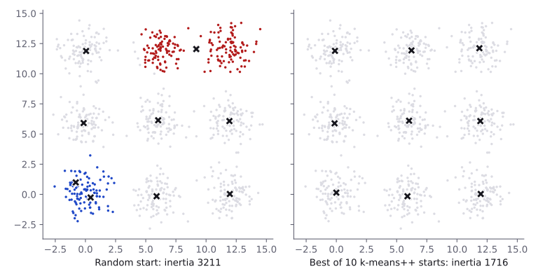
init="random" and n_init=1 (left) stops at a local minimum; ten k-means++ starts (right) place one centroid in each blob.Choosing the number of clusters
The number of clusters is a hyperparameter. Without labels it cannot be chosen by a validation score, and the smallest inertia falls whenever grows.
The elbow method plots the inertia against and chooses the value after which additional clusters reduce it only slightly.
Thus is near 1 when sample is much closer to its own cluster than to any other, near 0 when it lies between two clusters, and negative when another cluster is closer. The distances are not squared. In the running example, is at distance from and from , so , and is its mean distance to , and . Hence .
from sklearn.metrics import silhouette_samples, silhouette_score

print(silhouette_samples(X, km.labels_).round(4))
# [0.6731 0.6022 0.4288 0.5013 0.6232 0.5995]
print(round(silhouette_score(X, km.labels_), 4))  # 0.5713
The next code applies both heuristics to 600 samples drawn from four blobs.
Xc, yc = make_blobs(n_samples=600, centers=4, random_state=42)
for k in range(1, 8):
    km_c = KMeans(n_clusters=k, n_init=10, random_state=0).fit(Xc)
    sil = silhouette_score(Xc, km_c.labels_) if k > 1 else float("nan")
print(k, round(km_c.inertia_, 1), round(sil, 3))| 1 | 2 | 3 | 4 | 5 | 6 | 7 | |
|---|---|---|---|---|---|---|---|
| Inertia | 39698.3 | 18637.9 | 4178.9 | 1160.3 | 1045.8 | 938.4 | 844.2 |
| Silhouette score | — | 0.591 | 0.757 | 0.788 | 0.691 | 0.559 | 0.427 |
From 3 to 4 clusters the inertia falls by a factor of 3.6 and afterwards by only about 10% per cluster, so the elbow is at , where the silhouette score is also highest.
Comparing clusters with known labels
When labels are known, clusters are compared with them by the adjusted Rand index (ARI), adjusted_rand_score. The Rand index is the fraction of pairs of samples that two groupings treat alike, placing both samples together or both apart. The ARI corrects it for chance, so that random assignments score about 0 and identical groupings score 1 however the clusters are numbered.
from sklearn.datasets import load_iris
from sklearn.metrics import adjusted_rand_score

iris = load_iris()
for k in range(2, 6):
    labels = KMeans(n_clusters=k, n_init=10,
                    random_state=0).fit_predict(iris.data)
    print(k, round(silhouette_score(iris.data, labels), 3),
          round(adjusted_rand_score(iris.target, labels), 3))
print(adjusted_rand_score([0, 0, 1, 1], [1, 1, 0, 0])) # 1.0| Silhouette score | ARI with the species | |
|---|---|---|
| 2 | 0.681 | 0.54 |
| 3 | 0.553 | 0.73 |
| 4 | 0.498 | 0.65 |
| 5 | 0.489 | 0.608 |
The silhouette score prefers , which separates the 50 setosa and 3 versicolor flowers from the overlapping versicolor and virginica flowers; the species are matched best at . Well-separated groups need not be classes, so both heuristics are guides, not rules.
Scaling and cluster shape
Scaling
As in K-NN, a feature with a large range dominates Euclidean distances, and standardisation gives the features equal weight. The six people below fall into two groups by height, and their incomes, a second feature, have nothing to do with the groups.
| Person | Height (m) | Income |
|---|---|---|
| 0 | 1.58 | 52,000 |
| 1 | 1.61 | 31,000 |
| 2 | 1.63 | 66,000 |
| 3 | 1.79 | 38,000 |
| 4 | 1.81 | 59,000 |
| 5 | 1.84 | 45,000 |
import pandas as pd
from sklearn.pipeline import make_pipeline
from sklearn.preprocessing import StandardScaler

people = pd.DataFrame({
    "height_m": [1.58, 1.61, 1.63, 1.79, 1.81, 1.84],
    "income": [52_000, 31_000, 66_000, 38_000, 59_000, 45_000],
})
kmeans = KMeans(n_clusters=2, n_init=10, random_state=0)
raw = kmeans.fit_predict(people)
scaled = make_pipeline(StandardScaler(), kmeans).fit_predict(people)
print(raw, scaled) # [1 0 1 0 1 0] [1 1 1 0 0 0]| Person | Height (m) | Income | Cluster, raw | Cluster, scaled |
|---|---|---|---|---|
| 0 | 1.58 | 52,000 | 1 | 1 |
| 1 | 1.61 | 31,000 | 0 | 1 |
| 2 | 1.63 | 66,000 | 1 | 1 |
| 3 | 1.79 | 38,000 | 0 | 0 |
| 4 | 1.81 | 59,000 | 1 | 0 |
| 5 | 1.84 | 45,000 | 0 | 0 |
On the raw features, a difference of a few thousand in income outweighs any difference in height, so the clusters split the people into lower and higher incomes and ignore height. After standardising, both features count equally, and the clusters match the two height groups. The same happens with more data: for 200 people generated in a similar way, the adjusted Rand index with the height groups is 0.007 without scaling and 1.0 with it. Scaling is still a modelling decision: on Iris, whose features are all lengths in centimetres, standardising lowers the ARI of three clusters from 0.73 to 0.62.
Cluster shape
Each sample joins its nearest centroid, so the boundary between two clusters is the set of points equidistant from their centroids, and every cluster is a convex region. The User Guide adds that inertia assumes isotropic clusters, equally spread in all directions. K-means therefore fails on curved or elongated groups.
from sklearn.cluster import DBSCAN
from sklearn.datasets import make_moons
from sklearn.mixture import GaussianMixture

Xm, ym = make_moons(n_samples=400, noise=0.05, random_state=0)
moons = KMeans(n_clusters=2, n_init=10, random_state=0).fit(Xm)
print(round(adjusted_rand_score(ym, moons.labels_), 3))  # 0.274

Xa, ya = make_blobs(n_samples=600, centers=3, random_state=170)
Xa = Xa @ np.array([[0.6, -0.6], [-0.4, 0.8]])   # stretch the blobs
aniso = KMeans(n_clusters=3, n_init=10, random_state=0).fit(Xa)
true_J = sum(((Xa[ya == j] - Xa[ya == j].mean(axis=0)) ** 2).sum()
             for j in range(3))
print(round(adjusted_rand_score(ya, aniso.labels_), 3))  # 0.58
print(round(aniso.inertia_, 1), round(true_J, 1))  # 690.8 876.9

db = DBSCAN(eps=0.2).fit_predict(Xm)
gm = GaussianMixture(n_components=3, random_state=0).fit_predict(Xa)
print(round(adjusted_rand_score(ym, db), 3),
      round(adjusted_rand_score(ya, gm), 3))  # 1.0 1.0
The ARI is 0.274 on two interleaving half-moons and 0.58 on three stretched blobs. For the blobs, the K-means clustering even has a lower inertia than the true groups, 690.8 against 876.9: the objective, not its optimisation, is at fault. Other methods make other assumptions:
DBSCANbuilds clusters from samples connected through dense neighbourhoods and needs no . It separates the moons witheps=0.2, but with its defaulteps=0.5it puts all 400 samples in one cluster.GaussianMixturemodels each cluster as a Gaussian distribution with its own covariance matrix and recovers the stretched blobs exactly.
In scikit-learn
KMeans in sklearn.cluster follows the estimator interface, with fit taking only X.
| Parameter | Default | Meaning |
|---|---|---|
n_clusters |
8 |
The number of clusters |
init |
"k-means++" |
"k-means++", "random" or an array of starting centroids |
n_init |
"auto" |
Number of starts: 1 for "k-means++" or an array, 10 for "random" |
max_iter |
300 |
Maximum number of iterations per start |
tol |
1e-4 |
Stop when the total squared movement of the centroids is at most tol times the mean feature variance |
algorithm |
"lloyd" |
"elkan" skips distance computations using the triangle inequality, at a higher memory cost |
random_state |
None |
Seed for the initialisation |
km_iris = KMeans(n_clusters=3, random_state=0).fit(iris.data)
print(km_iris.cluster_centers_.round(2))  # one row per cluster
# [[5.88 2.74 4.39 1.43]
#  [5.01 3.43 1.46 0.25]
#  [6.85 3.08 5.72 2.05]]
print(km_iris.labels_[:5], np.bincount(km_iris.labels_))
# [1 1 1 1 1] [61 50 39]
print(round(km_iris.inertia_, 2), km_iris.n_iter_)  # 78.86 7

new = np.array([[5.0, 3.4, 1.5, 0.2], [6.5, 3.0, 5.5, 2.0]])
print(km_iris.predict(new))              # [1 2]
print(km_iris.transform(new).round(2))   # distance to each centroid
# [[3.33 0.07 4.97]
#  [1.42 4.67 0.42]]
print(np.isclose(km_iris.score(iris.data), -km_iris.inertia_))  # True
predict assigns samples to the nearest fitted centroid, transform returns their distances to all centroids as an array of shape (n_samples, n_clusters), and score returns minus the inertia.
MiniBatchKMeans updates the centroids from random batches of batch_size samples (default 1024), and partial_fit processes data in chunks. The User Guide states that it converges faster than KMeans, usually with a small loss in quality; the actual speed-up depends on the data, so it should be measured on the task at hand.
From scratch in NumPy
The function below implements the algorithm box, computing all squared distances at once by broadcasting.
def lloyd(X, centroids, max_iter=300):
    centroids = centroids.astype(float)          # a copy
    labels = None
    for _ in range(max_iter):
        # Squared distance from every sample to every centroid: (n, k)
        d2 = ((X[:, None, :] - centroids[None, :, :]) ** 2).sum(axis=2)
        new_labels = d2.argmin(axis=1)
        if labels is not None and (new_labels == labels).all():
            break                                # no sample moved
        labels = new_labels
        for j in range(len(centroids)):
            if (labels == j).any():              # empty: keep centroid
                centroids[j] = X[labels == j].mean(axis=0)
    inertia = ((X - centroids[labels]) ** 2).sum()
    return centroids, labels, inertia

start3 = iris.data[[0, 50, 100]]    # one flower of each species
c, lab, J = lloyd(iris.data, start3)
sk = KMeans(n_clusters=3, init=start3, n_init=1, tol=0).fit(iris.data)
print(np.allclose(c, sk.cluster_centers_), (lab == sk.labels_).all())
# True True
print(round(J, 4), round(sk.inertia_, 4))    # 78.8514 78.8514
From the same start, it returns the same centroids, labels and inertia as KMeans with tol=0, which disables the early stop on centroid movement. An empty cluster keeps its centroid here, whereas scikit-learn relocates it.
K-means in practice
Distances as features
transform describes each sample by its distances to the centroids. These distances are non-linear functions of the original features, so a linear model can use them to follow a curved boundary. Inside a pipeline, the centroids are fitted on the training data only.
from sklearn.linear_model import LogisticRegression
from sklearn.model_selection import train_test_split

Xn, yn = make_moons(n_samples=1000, noise=0.2, random_state=0)
Xn_tr, Xn_te, yn_tr, yn_te = train_test_split(
    Xn, yn, test_size=0.3, stratify=yn, random_state=0)
linear = LogisticRegression().fit(Xn_tr, yn_tr)
print(round(linear.score(Xn_te, yn_te), 3))          # 0.87

with_distances = make_pipeline(
    KMeans(n_clusters=20, random_state=0),   # 20 distance features
    StandardScaler(), LogisticRegression())
with_distances.fit(Xn_tr, yn_tr)
print(round(with_distances.score(Xn_te, yn_te), 3))  # 0.97
On noisy half-moons, logistic regression reaches a test accuracy of 0.87 on the two raw features and 0.97 on the 20 distances. In Lost in Hyperspace (IOAI 2024), whose model was fixed to linear regression, the rules banned supervised feature extractors but allowed unsupervised learning.
A few labelled samples
When only a few samples are labelled, clusters fitted to all samples can pass the labels on: each cluster takes the majority label of its labelled samples. The code draws one labelled sample per Wine cultivar, 20 times.
from collections import Counter
from sklearn.datasets import load_wine

wine = load_wine()
W_tr, W_te, w_tr, w_te = train_test_split(
    wine.data, wine.target, test_size=0.3, stratify=wine.target,
    random_state=0)
clusterer = make_pipeline(
    StandardScaler(), KMeans(n_clusters=3, n_init=10, random_state=0))
clusters = clusterer.fit_predict(W_tr)       # all 124 training rows
test_clusters = clusterer.predict(W_te)

sup_acc, ctl_acc = [], []
for seed in range(20):
    r = np.random.default_rng(seed)
    known = [r.choice(np.flatnonzero(w_tr == c)) for c in range(3)]
    # Supervised model trained on the three labelled rows only
    sup = make_pipeline(StandardScaler(), LogisticRegression())
    sup.fit(W_tr[known], w_tr[known])
    sup_acc.append(sup.score(W_te, w_te))
    # Each cluster takes the majority label of its labelled rows
    votes = [Counter(w_tr[i] for i in known if clusters[i] == c)
             for c in range(3)]
    if all(votes):
        mapping = np.array([v.most_common(1)[0][0] for v in votes])
        ctl_acc.append((mapping[test_clusters] == w_te).mean())
print(round(np.mean(sup_acc), 3), round(min(sup_acc), 3),
      round(max(sup_acc), 3))                # 0.722 0.315 0.926
print(len(ctl_acc), round(np.mean(ctl_acc), 3))  # 18 0.944
Logistic regression trained on the three labelled samples reaches a mean test accuracy of 0.722, between 0.315 and 0.926. The labelled clusters reach 0.944 in the 18 draws in which every cluster receives a label.
Resources
| Source | Title | Why read it |
|---|---|---|
| scikit-learn | User Guide: Clustering | Read “K-means” and “Mini Batch K-Means” for the algorithm and its assumptions, and “Rand index” and “Silhouette Coefficient” under “Clustering performance evaluation”. |
| scikit-learn | KMeans | Every parameter with its default, including init and n_init, and the fitted attributes cluster_centers_, labels_, inertia_ and n_iter_. |
| scikit-learn | Demonstration of k-means assumptions | K-means on anisotropic blobs, blobs of unequal variance and unevenly sized blobs, with remedies under “Possible solutions”. |
| scikit-learn | Selecting the number of clusters with silhouette analysis on KMeans clustering | Silhouette plots for 2 to 6 clusters on synthetic blobs, and how to read them. |
| James et al. | An Introduction to Statistical Learning with Python, section 12.4 | Free book. Section 12.4.1, “K-Means Clustering”, shows that the algorithm reaches a local optimum and compares six random starts; section 12.4.3, “Practical Issues in Clustering”, discusses standardisation and the robustness of clusters. |
| Stanford CS229 | Lecture notes: The k-means clustering algorithm | Three pages showing that k-means is coordinate descent on the distortion function J, which therefore decreases monotonically but can stop at a local optimum. |
| Arthur and Vassilvitskii | k-means++: The Advantages of Careful Seeding | The paper that introduced k-means++. Section 2.2 defines the D² weighting, and Theorem 3.1 bounds the expected inertia by 8(ln k + 2) times the optimum. |
| Google for Developers | Clustering course: Advantages and disadvantages of k-means | “Disadvantages of k-means” covers the manual choice of k, the dependence on initial values, outliers and high-dimensional data. |
| StatQuest | StatQuest: K-means clustering | Runs the algorithm step by step on a small example and shows how to choose k with an elbow plot. |
Practice problems
| Solved | Source | Problem | Difficulty | Tags |
|---|---|---|---|---|
| IOAI 2025 | Antique Painting Authentication | Medium | tabular, semi-supervised, clustering |