4Classical Machine Learning 4.5Classical Machine Learning Theory
4.5.5Cross-Validation
Estimating performance on new data by fitting and scoring a model on several complementary splits of the labelled data, with splitters for classes, groups and time order.
When two models are compared on a single validation set, part of the difference is luck. A different split of the same data could have put a few harder samples on the other side and picked a different winner. With a small dataset, that luck can be larger than the real difference between the models.
This is one of the easiest ways to fool yourself in a contest: a change seems to improve the validation score, but the improvement is only noise, and the model does no better on the hidden test set. The more models and settings you compare, the more likely this becomes.
Cross-validation is the standard way to take that luck out of model comparisons and hyperparameter choices, and it is worth using whenever labelled data is limited and the training time allows it.
A validation set estimates performance on new data, but the estimate from one split is noisy, as the comparison of candidates in Approaching a Typical Problem shows. Cross-validation fits and scores a model on several complementary splits of the labelled data and averages the scores. Scikit-learn Basics shows a first call to cross_val_score. This module covers how the splits are formed, how to evaluate a hyperparameter search, and the cost of cross-validation in contests.
Why one split is not enough
The experiment below keeps the model fixed, logistic regression on standardised features of the Breast Cancer dataset, and changes only the validation samples. StratifiedShuffleSplit draws 100 independent random splits, each holding out a stratified 20%, or 114 samples. For comparison, 5-fold cross-validation, defined in the next section, is run with 100 different shuffles.
import numpy as np
from sklearn.datasets import load_breast_cancer
from sklearn.linear_model import LogisticRegression
from sklearn.model_selection import (
    StratifiedKFold, StratifiedShuffleSplit, cross_val_score)
from sklearn.pipeline import make_pipeline
from sklearn.preprocessing import StandardScaler

X, y = load_breast_cancer(return_X_y=True)  # 569 samples
model = make_pipeline(StandardScaler(), LogisticRegression())

# 100 random stratified 80/20 splits: one validation score each
splits = StratifiedShuffleSplit(
    n_splits=100, test_size=0.2, random_state=0)
single = cross_val_score(model, X, y, cv=splits)

# 100 runs of 5-fold cross-validation, each with its own shuffle
means = np.array([
    cross_val_score(model, X, y, cv=StratifiedKFold(
        5, shuffle=True, random_state=seed)).mean()
    for seed in range(100)
])
for name, s in [("one split", single), ("5-fold mean", means)]:
    print(f"{name:12} min {s.min():.3f}  max {s.max():.3f}"
          f"  std {s.std():.4f}")
# one split    min 0.939  max 1.000  std 0.0121
# 5-fold mean  min 0.968  max 0.984  std 0.0034
The accuracy on a single split ranges from 0.939 to 1.000, a difference of 7 of the 114 validation samples, so two models compared on one split can differ by several points because of the split alone. The 5-fold mean ranges only from 0.968 to 0.984, and its standard deviation is less than a third of that of a single split, because each run validates all 569 samples instead of 114. Random splits, drawn by StratifiedShuffleSplit or its unstratified version ShuffleSplit, can overlap and may leave some samples unvalidated; the folds of -fold cross-validation cannot.
K-fold cross-validation
Without shuffling, KFold forms the folds from consecutive samples. For and , the code prints the rows of the table below; split yields row indices, not data.
from sklearn.model_selection import KFold

samples = np.arange(10)
for j, (train_idx, val_idx) in enumerate(KFold(5).split(samples)):
print(j + 1, train_idx, val_idx)| Fit | Training samples | Validation fold |
|---|---|---|
| 1 | 2, 3, 4, 5, 6, 7, 8, 9 | 0, 1 |
| 2 | 0, 1, 4, 5, 6, 7, 8, 9 | 2, 3 |
| 3 | 0, 1, 2, 3, 6, 7, 8, 9 | 4, 5 |
| 4 | 0, 1, 2, 3, 4, 5, 8, 9 | 6, 7 |
| 5 | 0, 1, 2, 3, 4, 5, 6, 7 | 8, 9 |
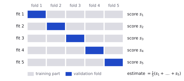
function cross_validate(model, X, y, k, metric):
    folds = the row indices, split into k parts of nearly equal size
    scores = []
    for each fold in folds:
        train = all rows that are not in fold
        fitted = fresh copy of model, fitted on X[train], y[train]
        scores.append(metric(y[fold], fitted.predict(X[fold])))
    return mean(scores), std(scores)
The loop below implements the algorithm and agrees with cross_val_score. It is shown only to make the algorithm concrete: in a contest, a hand-written loop like this is almost never needed, and cross_val_score or cross_validate should be used instead. clone returns an unfitted copy with the same hyperparameters.
from sklearn.base import clone

cv = StratifiedKFold(5, shuffle=True, random_state=0)
scores = []
for train_idx, val_idx in cv.split(X, y):
    fold_model = clone(model)  # a new, unfitted copy
    fold_model.fit(X[train_idx], y[train_idx])
    scores.append(fold_model.score(X[val_idx], y[val_idx]))
scores = np.array(scores)

print(scores.round(3))  # [0.956 0.974 0.982 1.    0.982]
print(np.allclose(scores, cross_val_score(model, X, y, cv=cv)))
# True
print(round(scores.mean(), 3), round(scores.std(), 3))  # 0.979 0.014
The folds contain 114, 114, 114, 114 and 113 samples, and the result is reported as , the mean and standard deviation of the fold scores. Models that are compared should be scored on the same folds, by passing the same cv object to each.
Choosing k
Each fold model is trained on a fraction of the labelled data, and fits are needed. The code runs -fold cross-validation with 20 shuffles for each value of .
for k in [2, 3, 5, 10, 20]:
    runs = [cross_val_score(model, X, y, cv=StratifiedKFold(
                k, shuffle=True, random_state=seed)).mean()
            for seed in range(20)]
print(k, round(np.mean(runs), 4), round(np.std(runs), 4))| Fits | Training samples per fit | Mean estimate | Standard deviation over shuffles | |
|---|---|---|---|---|
| 2 | 2 | 284–285 | 0.9755 | 0.0041 |
| 3 | 3 | 379–380 | 0.9768 | 0.0040 |
| 5 | 5 | 455–456 | 0.9790 | 0.0030 |
| 10 | 10 | 512–513 | 0.9788 | 0.0026 |
| 20 | 20 | 540–541 | 0.9793 | 0.0020 |
With , each model sees half of the data, and the estimate is 0.0035 lower than with : too few training samples make it pessimistic. Beyond , the estimate changes by less than 0.001 while the cost keeps growing. The usual choices are , the scikit-learn default, and when fits are cheap.
Stratification and shuffling
When cv is an integer or is omitted, scikit-learn uses StratifiedKFold for a classifier with binary or multi-class labels, including a pipeline that ends in a classifier, and KFold otherwise, both without shuffling. Stratified folds keep the class proportions of the whole dataset, for the reason given in Approaching a Typical Problem. Unshuffled folds follow the row order, which matters for a sorted file such as Iris.
from sklearn.datasets import load_iris

X_iris, y_iris = load_iris(return_X_y=True)
print(y_iris[:3], y_iris[50:53], y_iris[100:103])
# [0 0 0] [1 1 1] [2 2 2]: the rows are sorted by species

for cv_iris in [KFold(3), StratifiedKFold(3),
                KFold(3, shuffle=True, random_state=0)]:
    print(cross_val_score(model, X_iris, y_iris, cv=cv_iris).round(2))
# [0. 0. 0.]
# [0.98 0.96 0.96]
# [0.94 0.96 0.96]
With KFold(3), each fold is exactly one species. Every model is validated on a species absent from its training data, so all its predictions are wrong. StratifiedKFold(3) places about a third of each species in every fold, and shuffling mixes the rows before splitting; both score about 0.96.
Stratification does not remove other orderings: without shuffling, StratifiedKFold takes each class in file order (setosa rows 0–16, 17–33 and 34–49 in the three Iris folds), so a file also sorted by date or source gives folds that differ in that variable. When the row order carries no meaning, shuffle=True with a fixed random_state gives mixed and reproducible folds; when it does, the splitters of the next section apply.
Groups and time order
A cross-validation estimate is reliable only if each validation fold relates to its training part as the hidden test data relates to the training data. Random folds break this in two common cases.
Grouped samples
Six measurements from three patients show the difference. Each patient contributes two measurements, and each splitter puts every measurement into one of three validation folds:
from sklearn.model_selection import GroupKFold

patient = np.array([0, 0, 1, 1, 2, 2])  # patient of each measurement
X_six = np.zeros((6, 1))                # the features do not matter
folds = {}
for splitter in [KFold(3, shuffle=True, random_state=0), GroupKFold(3)]:
    fold = np.empty(6, dtype=int)
    for j, (_, val) in enumerate(splitter.split(X_six, groups=patient)):
        fold[val] = j + 1               # the fold that validates it
folds[type(splitter).__name__] = fold| Measurement | 1 | 2 | 3 | 4 | 5 | 6 |
|---|---|---|---|---|---|---|
| Patient | 0 | 0 | 1 | 1 | 2 | 2 |
Validation fold with shuffled KFold |
3 | 2 | 1 | 2 | 3 | 1 |
Validation fold with GroupKFold |
3 | 3 | 2 | 2 | 1 | 1 |
With shuffled KFold, the two measurements of every patient land in different folds, so each patient is validated by a model that was trained on that patient's other measurement. GroupKFold keeps both measurements of a patient in the same fold.
Samples from one source resemble each other, so if the test data comes from new sources, a model validated on sources seen in training can score well by recognising the source instead of learning how the label depends on the features. The synthetic data below has 100 patients with 10 measurements each. Each patient has its own profile of five features, the label belongs to the patient, and only feature 0 depends on the label.
from sklearn.neighbors import KNeighborsClassifier

def make_patients(n_patients, rng):
    # 10 measurements per patient; the label belongs to the patient
    label = rng.permutation(np.arange(n_patients) % 2)
    centre = rng.normal(size=(n_patients, 5))  # the patient's profile
    centre[:, 0] += 3 * label                  # the real signal
    groups = np.repeat(np.arange(n_patients), 10)
    noise = rng.normal(scale=0.3, size=(len(groups), 5))
    return centre[groups] + noise, label[groups], groups

rng = np.random.default_rng(0)
X_p, y_p, patient = make_patients(100, rng)   # 1,000 samples
X_new, y_new, _ = make_patients(1000, rng)    # 10,000 new samples

knn = KNeighborsClassifier()
shuffled = KFold(5, shuffle=True, random_state=0)
print(round(cross_val_score(knn, X_p, y_p, cv=shuffled).mean(), 3))
print(round(cross_val_score(knn, X_p, y_p, cv=GroupKFold(5),
                            groups=patient).mean(), 3))
print(round(knn.fit(X_p, y_p).score(X_new, y_new), 3))
# 0.979
# 0.881
# 0.878
Shuffled KFold estimates an accuracy of 0.979, but the accuracy on 1,000 new patients is 0.878. Most measurements of a validated patient remain in the training part, and 79% of the five nearest neighbours of a measurement belong to the same patient, so K-NN largely recognises patients. GroupKFold validates each patient with a model that has seen none of that patient's measurements, and its estimate, 0.881, is close to the accuracy on new patients. StratifiedGroupKFold also keeps the class proportions of the folds similar, as far as whole groups allow.
The splitter should imitate the difference between training and test data that the task statement describes.
- Find the Order (IOAI 2026): each of the 1,288 training dialogues is cut into 7 to 20 speaker-turn audio clips, and the test sets consist of held-out dialogues. A model trained on clips, or on pairs of clips, should be validated with dialogues as groups.
- Robot Delivery Academy (IOAI 2026 At-Home Round): the 5,327 training state–action samples come from 400 expert demonstrations, and evaluation uses scenarios that were not shown as demonstrations, so the demonstrations are the groups.
- Robot Chasing (IOAI 2026): the rows are independent snapshots, and the same six robots appear in the training data and in the public test set. Holding out whole robots would validate on robots that the test data never introduces.
Time order
When a model must predict later samples from earlier ones, a random fold trains it partly on samples recorded after those it validates, which is impossible in actual use. TimeSeriesSplit trains on an initial segment of the rows, sorted by time, and validates on the segment that follows.
from sklearn.model_selection import TimeSeriesSplit

for train_idx, val_idx in TimeSeriesSplit(3).split(np.arange(12)):
    print(train_idx, val_idx)
# [0 1 2] [3 4 5]
# [0 1 2 3 4 5] [6 7 8]
# [0 1 2 3 4 5 6 7 8] [ 9 10 11]
Every validation sample comes after all of its training samples. The first segment is never validated. The gap argument drops a given number of samples from the end of each training segment, which separates it from the validation segment when neighbouring samples are strongly correlated.
Preprocessing inside the folds
Every step that learns from data, such as scaling, imputation or feature selection, is part of training and must be refitted in each fold. Fitting it on all labelled data first is the data leakage demonstrated in Approaching a Typical Problem. Passing the whole pipeline to the cross-validation function avoids it, as the fitted pipelines returned by cross_validate, described in the next section, show.
from sklearn.model_selection import cross_validate

res = cross_validate(model, X, y, cv=cv, return_estimator=True)
for fitted in res["estimator"]:
    print(fitted.named_steps["standardscaler"].mean_[:2].round(2))
print(X[:, :2].mean(axis=0).round(2))  # all 569 samples
# [14.15 19.36]
# [14.12 19.19]
# [14.14 19.16]
# [14.12 19.33]
# [14.09 19.4 ]
# [14.13 19.29]
Each scaler learned its means from its own 455 or 456 training samples; a scaler fitted before cross-validation would use the means over all 569 samples, printed last, in every fold. A transformation computed from each sample alone, such as the logarithm of a feature, learns nothing from other samples and can be applied before splitting.
More cross-validation tools
cross_validate returns a dictionary with the fit and scoring times and one array of fold scores per metric. scoring accepts a list of the scorer names described in Model Evaluation Metrics, and return_train_score=True adds the scores on the training parts.
from sklearn.ensemble import RandomForestClassifier

forest = RandomForestClassifier(random_state=0)
res = cross_validate(
    forest, X, y, cv=cv, return_train_score=True,
    scoring=["accuracy", "balanced_accuracy", "roc_auc"])
print(list(res))
# ['fit_time', 'score_time', 'test_accuracy', 'train_accuracy',
#  'test_balanced_accuracy', 'train_balanced_accuracy', 'test_roc_auc',
#  'train_roc_auc']
for key in ["test_accuracy", "test_roc_auc", "train_accuracy"]:
    print(key, round(res[key].mean(), 3))
# test_accuracy 0.965
# test_roc_auc 0.992
# train_accuracy 1.0
The forest fits its training parts perfectly but reaches 0.965 on the validation folds, a gap analysed in Underfitting and Overfitting.
cross_val_predict returns out-of-fold predictions: each sample is predicted by the model whose validation fold contained it, so no prediction comes from a model that saw the sample.
from sklearn.metrics import confusion_matrix
from sklearn.model_selection import cross_val_predict

oof = cross_val_predict(model, X, y, cv=cv)
print(oof.shape)                 # (569,)
print(confusion_matrix(y, oof))  # rows: true class 0, then 1
# [[203   9]
#  [  3 354]]
Label 0 is malignant in load_breast_cancer, so 9 of the 212 malignant tumours are predicted benign and 3 of the 357 benign ones malignant. Out-of-fold probabilities, from method="predict_proba", can be used to choose a decision threshold. The scikit-learn documentation warns that a metric computed from pooled out-of-fold predictions is not always a valid measure of generalisation: it differs from the mean fold score unless all folds have equal size and the metric is an average over samples.
RepeatedStratifiedKFold repeats stratified -fold cross-validation with a new shuffle each time.
from sklearn.model_selection import RepeatedStratifiedKFold

rcv = RepeatedStratifiedKFold(n_splits=5, n_repeats=10, random_state=0)
scores = cross_val_score(model, X, y, cv=rcv)
print(len(scores), round(scores.mean(), 4))  # 50 0.9772
Averaging 50 scores makes the estimate steadier: across different shuffles its standard deviation is about 0.001, against 0.003 for a single 5-fold run, at ten times the cost. LeaveOneOut is -fold cross-validation with : it needs one fit per sample, 569 here, and each fold's accuracy is either 0 or 1.
Nested cross-validation
After a search, best_score_ is the highest of many cross-validated means, and the maximum of noisy estimates is biased upwards, as Hyperparameter Tuning shows. Nested cross-validation estimates the performance of the whole selection procedure instead. An outer cross-validation holds out each outer fold in turn, runs the complete search with its own inner folds on the remaining data, and scores the selected model on the held-out fold. Passing a GridSearchCV object to cross_val_score does exactly this.
from sklearn.model_selection import GridSearchCV
from sklearn.tree import DecisionTreeClassifier

tree = DecisionTreeClassifier(random_state=0)
grid = {"max_depth": [1, 2, 3, 4, 5, 6, None],
        "min_samples_leaf": [1, 5, 10, 20]}

gaps = []
for seed in range(10):
    inner = StratifiedKFold(5, shuffle=True, random_state=seed)
    outer = StratifiedKFold(5, shuffle=True, random_state=100 + seed)
    search = GridSearchCV(tree, grid, cv=inner)
    best = search.fit(X, y).best_score_            # not nested
    nested = cross_val_score(search, X, y, cv=outer).mean()
    gaps.append(best - nested)

print(round(min(gaps), 4), round(max(gaps), 4))  # -0.0071 0.0246
print(round(np.mean(gaps), 4), sum(g > 0 for g in gaps))  # 0.0083 8
Each of the 10 repetitions tunes 28 combinations of two decision tree hyperparameters with different fold seeds. best_score_ exceeds the nested estimate in 8 repetitions and by 0.0083 on average, although a single repetition can show the opposite. In the first repetition, the five outer searches selected four different combinations, so the nested estimate describes the procedure, not one setting. Each repetition costs fits.
Cross-validation in contests
-fold cross-validation costs fits, and a nested search many more, while an IOAI notebook must finish within the runtime limit of its task, often 5 to 20 minutes, as noted in Approaching a Typical Problem. Cross-validation therefore belongs to development, and the submitted notebook fits only the chosen model, as Hyperparameter Tuning recommends. Passing n_jobs=-1 runs the folds in parallel on all CPU cores.
The chosen model is usually refitted on all labelled data. Alternatively, the fold models can be kept and their test predictions averaged, which needs no further fit.
from sklearn.model_selection import train_test_split

X_lab, X_test, y_lab, y_test = train_test_split(
    X, y, test_size=0.2, stratify=y, random_state=0)
res = cross_validate(forest, X_lab, y_lab, cv=cv,
                     return_estimator=True)

# Option 1: refit the model on all labelled data
final = clone(forest).fit(X_lab, y_lab)
print(round(final.score(X_test, y_test), 3))  # 0.947

# Option 2: average the probabilities of the five fold models
proba = np.mean([m.predict_proba(X_test)[:, 1]
                 for m in res["estimator"]], axis=0)
print(round(((proba >= 0.5) == y_test).mean(), 3))  # 0.939
Here the two options differ by one of the 114 test samples. Either way, the official score comes from hidden data: under section 2.6 of the IOAI 2026 Contest Rules, submissions are scored during the contest on a validation dataset (Scoreboard A), but rankings use only a separate test dataset (Scoreboard B). Repeated adjustment to Scoreboard A overfits it, so cross-validation on the training data remains an independent check.
Resources
| Source | Title | Why read it |
|---|---|---|
| scikit-learn | User Guide: Cross-validation: evaluating estimator performance | “Cross validation iterators” describes every splitter in this module, including “Cross-validation iterators for grouped data” and “Cross validation of time series data”; “Obtaining predictions by cross-validation” covers cross_val_predict. |
| scikit-learn | Visualizing cross-validation behavior in scikit-learn | Plots the training and validation indices of KFold, GroupKFold, StratifiedKFold, TimeSeriesSplit and other splitters on the same data. |
| scikit-learn | Nested versus non-nested cross-validation | Compares the two estimates over repeated trials on the Iris dataset. |
| StatQuest | Machine Learning Fundamentals: Cross Validation | A short visual introduction to dividing data into folds and comparing methods by their cross-validated performance. |
| IOAI | 2026 Contest Rules and Technical Appendix | Section 2.6, “Feedback (Scoreboard)”, defines the training, validation and test datasets of a task and the scoreboards computed from them. |
Practice problems
| Solved | Source | Problem | Difficulty | Tags |
|---|---|---|---|---|
| IOAI 2026 | Robot Delivery Academy | Medium | imitation learning, grouped samples | |
| IOAI 2026 | Find the Order | Hard | audio, grouped samples |