4Classical Machine Learning 4.5Classical Machine Learning Theory
4.5.3Loss Functions
The functions that training minimises: regression and classification losses, their robustness and probabilistic meaning, sample and class weights, and their names in scikit-learn and XGBoost.
When a model trains, it needs a single number that says how wrong its current predictions are, so that it can adjust its parameters to make that number smaller. That number is the loss. Every model you have met so far has one, even where it was not named: linear regression minimises the squared error, and logistic regression minimises the log loss.
Choosing a loss is a real modelling decision, not a technical detail. The same model trained with two different losses can learn quite different things from the same data: one version aims at the average label and another at the median label, and a single extreme label can pull the first far more than the second.
Most of the time a model's default loss is a sensible choice. This module helps you recognise when it is not, for example when the labels contain outliers, when some mistakes cost more than others, or when the task's metric rewards something that the default loss does not.
A model is trained by choosing the parameters that minimise a loss function on the training data, as introduced in Terminology, and it is judged by a metric, which often differs from the loss. This module compares the common losses, relates them to assumptions about noise, shows how weights enter a loss, and gives their names in scikit-learn and XGBoost.
Loss, cost and objective
Here is the model's prediction for sample , is a penalty such as the sum of squared weights, and sets its strength. The of Ridge and Lasso and the of logistic regression are such strengths. Many texts say "loss" for all three terms when the meaning is clear from context.
Three samples with labels 3, 5 and 10 and predictions 4, 5 and 7 give the following losses.
| Sample | Label | Prediction | Squared error | Absolute error |
|---|---|---|---|---|
| 1 | 3 | 4 | 1 | 1 |
| 2 | 5 | 5 | 0 | 0 |
| 3 | 10 | 7 | 9 | 3 |
The squared-error cost is , the mean squared error. The absolute-error cost is , the mean absolute error. Sample 3 accounts for 90% of the first cost and 75% of the second: squaring gives large errors a larger share.
Regression losses
The regression losses below are functions of the residual .
Squared error is the loss of least squares, treated in Linear Regression. The two branches of the Huber loss have equal values and slopes at , so the loss is differentiable everywhere. With , the pinball loss is half the absolute error.
The best constant prediction
The effect of a loss is clearest for a model that predicts one constant for every sample. Take the labels 2, 3, 4, 5 and 36, where 36 is an outlier. The code tries every constant from 0 to 40 in steps of 0.001 and keeps, for each loss, the one with the smallest average loss.
import numpy as np

y = np.array([2.0, 3.0, 4.0, 5.0, 36.0])
c = np.linspace(0, 40, 40001)       # candidate constants, step 0.001
R = y - c[:, None]                  # residuals: one row per constant
A = np.abs(R)
losses = {
    "squared": R ** 2,
    "absolute": A,
    "Huber, delta=3": np.where(A <= 3, 0.5 * R ** 2, 3 * (A - 1.5)),
    "pinball, tau=0.75": np.maximum(0.75 * R, -0.25 * R),
}
for name, L in losses.items():
    best = c[np.argmin(L.mean(axis=1))]
print(f"{name}: {best:.3f}")| Loss | Best constant | Which value of the labels it is |
|---|---|---|
| Squared error | 10 | the mean |
| Absolute error | 4 | the median |
| Huber, | 4.25 | between the median and the mean |
| Pinball, | 5 | the 0.75-quantile |
- Squared error is minimised by the mean, as shown in Decision Trees.
- Absolute error. Where it exists, the derivative of with respect to is the number of labels below minus the number above it. Moving towards the side with more labels therefore lowers the cost, and the minimum is where the two counts balance: at the median.
- Pinball loss. The derivative is times the number of labels below minus times the number above it. It changes sign where about a fraction of the labels lies below , at the -quantile of the labels.
- Huber loss lies between the two. As grows from 1 to 40, its minimiser moves from the median, 4, to the mean, 10.
Replacing the outlier 36 by 6 moves the mean from 10 to 4 but leaves the median at 4. Absolute error and the Huber loss are robust: a few extreme labels move their minimiser little. For models with features, squared error trains a model to predict the mean label of samples with similar features, absolute error their median and the pinball loss their -quantile, so models trained with and estimate a 90% prediction interval.
Outliers in a linear model
The labels below follow the line with noise, and 10 of the 100 labels are then lowered by 30.
from sklearn.linear_model import (
    HuberRegressor, LinearRegression, QuantileRegressor,
)

rng = np.random.default_rng(0)
x = rng.uniform(0, 10, size=100)
y = 2 * x + 1 + rng.normal(0, 1, size=100)  # true line: y = 2x + 1
bad = rng.choice(100, size=10, replace=False)
y[bad] -= 30                                # corrupt 10 labels
X = x.reshape(-1, 1)

models = [LinearRegression(), HuberRegressor(),
          QuantileRegressor(quantile=0.5, alpha=0)]
for model in models:
    model.fit(X, y)
    print(type(model).__name__, round(model.coef_[0], 3),
          round(model.intercept_, 3))
# LinearRegression 2.241 -3.4
# HuberRegressor 1.99 0.856
# QuantileRegressor 1.973 1.118| Model | Loss | Slope | Intercept |
|---|---|---|---|
| True line | — | 2 | 1 |
LinearRegression |
squared error | 2.241 | −3.400 |
HuberRegressor |
Huber | 1.990 | 0.856 |
QuantileRegressor(alpha=0) |
absolute error | 1.973 | 1.118 |
To reduce the large squared residuals of the corrupted samples, least squares lowers the whole line, and its intercept falls to −3.4. Both robust fits stay close to the true line. QuantileRegressor adds an L1 penalty with alpha=1.0 by default, so alpha=0 is needed for the pure pinball loss. HuberRegressor applies its threshold epsilon (default 1.35) to residuals divided by a scale that it estimates, so the threshold does not depend on the units of .
Names in scikit-learn and XGBoost
| Loss | Best constant | scikit-learn | XGBoost objective |
|---|---|---|---|
| Squared error | mean | LinearRegression; loss="squared_error" in SGDRegressor, HistGradientBoostingRegressor, GradientBoostingRegressor |
"reg:squarederror" (the default) |
| Absolute error | median | QuantileRegressor(quantile=0.5); loss="absolute_error" in HistGradientBoostingRegressor, GradientBoostingRegressor; criterion="absolute_error" in DecisionTreeRegressor |
"reg:absoluteerror" |
| Huber | between median and mean | HuberRegressor; loss="huber" in SGDRegressor, GradientBoostingRegressor |
"reg:pseudohubererror", a smooth variant, with huber_slope |
| Pinball | -quantile | QuantileRegressor(quantile=τ); loss="quantile" with quantile=τ in HistGradientBoostingRegressor or alpha=τ in GradientBoostingRegressor |
"reg:quantileerror" with quantile_alpha=τ |
Classification losses
For binary classification, this section codes the labels as . A linear classifier computes a real-valued score , returned by decision_function in scikit-learn, and predicts when and otherwise.
A score of 2.5 gives the margin 2.5 for a sample with label and for a sample with label . Each loss below is a function of the margin alone.
- 0–1 loss: 1 if and 0 otherwise; its average is the error rate. It is constant on each side of 0, so its derivative is zero wherever it exists and gives gradient-based training no direction. Training therefore minimises a continuous surrogate loss, such as the three below.
- Log loss: . With and labels coded as 0 and 1, it equals the binary cross-entropy derived in Logistic Regression.
- Hinge loss: , the loss of the linear support vector machine. It is the default loss of
SGDClassifier, andLinearSVCuses it withloss="hinge"(its default is the squared hinge loss). It is 0 for , so samples classified correctly with a margin of at least 1 do not affect the fit. - Exponential loss: , the loss minimised by AdaBoost. According to its documentation,
GradientBoostingClassifier(loss="exponential")recovers the AdaBoost algorithm.
| Margin | −2 | −1 | 0 | 0.5 | 1 | 2 |
|---|---|---|---|---|---|---|
| 0–1 loss | 1 | 1 | 1 | 0 | 0 | 0 |
| Log loss | 2.127 | 1.313 | 0.693 | 0.474 | 0.313 | 0.127 |
| Hinge loss | 3 | 2 | 1 | 0.5 | 0 | 0 |
| Exponential loss | 7.389 | 2.718 | 1 | 0.607 | 0.368 | 0.135 |
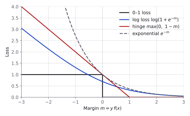
For large negative margins, the hinge and log losses grow linearly, but the exponential loss is multiplied by per unit, so a few badly misclassified samples, such as mislabelled ones, can dominate an exponential cost.
Scores and probabilities
Samples with identical features receive one common score . If a fraction of them has label , the code below finds the score that minimises their average loss.
f = np.linspace(-5, 5, 100001)          # candidate scores, step 0.0001
for p in [0.7, 0.9]:
    # average loss when a fraction p of the samples has y = +1
    log = p * np.log(1 + np.exp(-f)) + (1 - p) * np.log(1 + np.exp(f))
    hinge = p * np.maximum(0, 1 - f) + (1 - p) * np.maximum(0, 1 + f)
    f_log, f_hinge = f[np.argmin(log)], f[np.argmin(hinge)]
    p_back = 1 / (1 + np.exp(-f_log))
    print(p, round(f_log, 3), round(p_back, 3), round(f_hinge, 3))
# 0.7 0.847 0.7 1.0
# 0.9 2.197 0.9 1.0
Under log loss, the best score is the log-odds , 0.847 for and 2.197 for , and the sigmoid of that score recovers . Under hinge loss, the best score is 1 in both cases: it records which class is more frequent, but not by how much. A model trained with log loss therefore estimates probabilities, and a model trained with hinge loss only separates the classes.
from sklearn.datasets import load_breast_cancer
from sklearn.linear_model import SGDClassifier
from sklearn.model_selection import train_test_split
from sklearn.pipeline import make_pipeline
from sklearn.preprocessing import StandardScaler

X, y = load_breast_cancer(return_X_y=True)
X_train, X_test, y_train, y_test = train_test_split(
    X, y, test_size=0.2, stratify=y, random_state=0
)
for loss in ["hinge", "log_loss"]:
    clf = make_pipeline(StandardScaler(),
                        SGDClassifier(loss=loss, random_state=0))
    clf.fit(X_train, y_train)
    print(loss, round(clf.score(X_test, y_test), 3),
          hasattr(clf, "predict_proba"))
# hinge 0.965 False
# log_loss 0.965 True
Both models reach a test accuracy of 0.965, but only the log-loss model provides predict_proba. Likewise, the XGBoost documentation states that "binary:hinge" predicts 0 or 1 rather than probabilities, unlike "binary:logistic". For more than two classes, log loss becomes the cross-entropy of multinomial logistic regression, "multi:softprob" in XGBoost.
Losses as likelihoods
Logistic Regression obtains log loss as the negative logarithm of the likelihood, the probability that the model assigns to the observed labels. Squared and absolute error arise in the same way from assumptions about the noise in regression labels. Suppose that each label is the model's prediction plus independent random noise, .
- Gaussian noise. If has the normal density with standard deviation , the negative log-likelihood of one label is . The second term does not depend on the model, so maximising the likelihood is equivalent to minimising squared error.
- Laplace noise. If has the Laplace density with scale , the negative log-likelihood is , and maximising the likelihood is equivalent to minimising absolute error.
- Bernoulli labels. If each label is 1 with probability and 0 otherwise, the negative log-likelihood is log loss.
A loss is therefore an assumption about the noise. The Laplace density decreases more slowly: for and , a residual of 4 is times as probable as a residual of 0 under Laplace noise, but only times as probable under Gaussian noise. Absolute error therefore suits labels with occasional large errors.
Weighted losses
In scikit-learn, weights are passed as fit(X, y, sample_weight=w). For LogisticRegression, a weight of 2 gives the same model as including the sample twice:
from sklearn.linear_model import LogisticRegression

X, y = load_breast_cancer(return_X_y=True)
X = StandardScaler().fit_transform(X)
X_rep = np.vstack([X, X[:1]])         # sample 0 appears twice
y_rep = np.append(y, y[0])
w = np.ones(len(y))
w[0] = 2                              # sample 0 has weight 2

opts = dict(tol=1e-10, max_iter=10_000)
a = LogisticRegression(**opts).fit(X_rep, y_rep)
b = LogisticRegression(**opts).fit(X, y, sample_weight=w)
print(np.allclose(a.coef_, b.coef_),
      np.allclose(a.intercept_, b.intercept_))  # True True
Class weights
Classifiers also accept class_weight, which gives every sample of class the weight , multiplied by its sample_weight if one is given. With class_weight="balanced", scikit-learn uses
where is the number of classes and the number of training samples in class . Every class then has the same total weight, . In the training set below, 1,337 samples belong to class 0 and 163 to class 1, so and , and both classes have total weight 750.
from sklearn.datasets import make_classification
from sklearn.metrics import precision_score, recall_score
from sklearn.utils.class_weight import compute_class_weight

X, y = make_classification(
    n_samples=2000, n_features=10, n_informative=4, n_redundant=0,
    weights=[0.9], class_sep=1.5, random_state=0,
)
X_train, X_test, y_train, y_test = train_test_split(
    X, y, test_size=0.25, stratify=y, random_state=0
)
print(np.bincount(y_train))                      # samples per class
print(compute_class_weight("balanced", classes=np.array([0, 1]),
                           y=y_train).round(3))

for cw in [None, "balanced"]:
    clf = make_pipeline(StandardScaler(),
                        LogisticRegression(class_weight=cw))
    clf.fit(X_train, y_train)
    pred = clf.predict(X_test)
    print(cw, round(recall_score(y_test, pred), 3),
          round(precision_score(y_test, pred), 3))
# [1337  163]
# [0.561 4.601]
# None 0.204 0.846
# balanced 0.63 0.209
Without weights, the model finds only 20.4% of the positive test samples, a recall of 0.204. With balanced weights, the loss of a class-1 sample counts about 8.2 times as much as that of a class-0 sample, and the recall rises to 0.630. The precision, the fraction of positive predictions that are correct, falls from 0.846 to 0.209. Balanced accuracy rises from 0.600 to 0.670 and accuracy falls from 0.910 to 0.702, so whether weighting helps depends on the metric. Lowering the decision threshold of the unweighted model has a similar effect.
Choosing a loss
The training loss should agree with the metric by which the predictions are judged.
| Task metric | Training loss |
|---|---|
| MSE or RMSE | squared error |
| Mean absolute error | absolute error, or Huber loss with a small threshold |
| A quantile or a prediction interval | pinball loss at the required levels |
| Log loss, or any use of predicted probabilities | log loss |
| Accuracy, F1 or another metric of predicted classes | log loss or hinge loss, followed by a threshold chosen on validation data |
| A metric with sample or class weights | the loss with the same weights |
Accuracy, F1 and ROC AUC change only in steps as the parameters change, so gradient methods cannot minimise them. A surrogate loss is minimised instead, and the decision threshold is then tuned for the metric, as described in Model Evaluation Metrics.
- Decision trees choose splits by an impurity criterion. The regression criteria
"squared_error"and"absolute_error"correspond to the squared and absolute losses, with leaves that predict the mean and the median; the classification criteria are described in Decision Trees. - Gradient boosting fits each new tree to the negative gradient of the loss, so it works with most losses in this module, as described in XGBoost.
- Neural networks use the same losses, for example as
nn.MSELoss,nn.L1Lossandnn.CrossEntropyLossin PyTorch; the deep learning module on loss functions covers them.
Resources
| Source | Title | Why read it |
|---|---|---|
| scikit-learn | User Guide: Stochastic Gradient Descent | The section “Mathematical formulation” gives the formula of every loss available in SGDClassifier and SGDRegressor, including hinge, log loss and Huber. |
| scikit-learn | SGD: convex loss functions | A short script that plots the zero-one, hinge, log and other classification losses against the decision score of a sample with label 1. Its log loss uses base-2 logarithms. |
| scikit-learn | User Guide: Linear Models | The sections “Huber Regression” and “Quantile Regression” state the exact objectives of HuberRegressor and QuantileRegressor, including the scale estimate of the first and the L1 penalty of the second. |
| scikit-learn | HuberRegressor vs Ridge on dataset with strong outliers | Shows the Huber fit moving towards the ridge fit as epsilon increases. |
| Google for Developers | Linear regression: Loss | “Types of loss” and “Choosing a loss” compare squared and absolute loss and how each treats outliers. |
| XGBoost | XGBoost Parameters | “Learning Task Parameters” lists every objective string, followed by the parameters of the pseudo-Huber and quantile losses. |
Practice problems
| Solved | Source | Problem | Difficulty | Tags |
|---|---|---|---|---|
| IOAI 2025 | Radar (at-home) | Medium | segmentation, imbalanced classes | |
| IOAI 2025 | Chicken Counting | Hard | vision, regression |