4Classical Machine Learning 4.5Classical Machine Learning Theory
4.5.2Underfitting and Overfitting
How model complexity, bias and variance determine the gap between training and validation performance, and how validation curves and learning curves diagnose it.
Every model you train can fail in one of two opposite ways. It can be too simple to capture the pattern in the data, like a straight line fitted to a curve. Or it can be so flexible that it memorises the training data, noise included, and then does poorly on anything new, like a student who memorises past exam answers without understanding them.
Much of machine learning, from choosing a model to setting its hyperparameters, is about steering between these two failures. A deeper tree, more features or weaker regularisation move a model towards overfitting; a shallower tree, fewer features or stronger regularisation move it towards underfitting.
Recognising which failure you are facing is one of the most useful skills in a contest, because the fixes point in opposite directions: adding complexity helps an underfitting model and hurts an overfitting one.
Terminology defines underfitting as high error on both the training data and the validation data, and overfitting as low training error combined with substantially higher validation error. This module explains both through model complexity, splits the expected error into bias, variance and noise, and introduces two diagnostic tools, validation curves and learning curves. It closes with remedies and with overfitting to validation data.
Model complexity
Complexity is set by the choice of model and by hyperparameters such as the polynomial degree, the maximum depth of a decision tree or in K-NN. Its effect is clearest on a synthetic problem, whose true relationship is known.
In the following problem, each input is drawn uniformly from the interval , and its label is
where the noise is normally distributed with mean 0 and standard deviation . At , for example, , and each label drawn there is 1 plus independent noise. No model can predict the noise, so even has an expected squared error of on new data.
The code fits polynomials of degree , , to 25 training samples with polynomial features and least squares, and measures the mean squared error (MSE) on them and on 1,000 validation samples.
import numpy as np
from sklearn.linear_model import LinearRegression
from sklearn.metrics import mean_squared_error
from sklearn.pipeline import make_pipeline
from sklearn.preprocessing import PolynomialFeatures

rng = np.random.default_rng(0)

def f(x):
    return np.sin(np.pi * x)            # the true relationship

def sample(n, noise=0.3):
    # n inputs uniform on [-1, 1]; labels with Gaussian noise
    x = rng.uniform(-1, 1, n)
    return x.reshape(-1, 1), f(x) + rng.normal(0, noise, n)

def poly_model(degree):
    return make_pipeline(
        PolynomialFeatures(degree, include_bias=False),
        LinearRegression(),
    )

X_train, y_train = sample(25)
X_val, y_val = sample(1000)

for degree in [1, 2, 3, 4, 5, 6, 8, 10, 12, 15]:
    model = poly_model(degree).fit(X_train, y_train)
    train_mse = mean_squared_error(y_train, model.predict(X_train))
    val_mse = mean_squared_error(y_val, model.predict(X_val))
print(degree, round(train_mse, 3), round(val_mse, 3))| Degree | Training MSE | Validation MSE |
|---|---|---|
| 1 | 0.285 | 0.400 |
| 2 | 0.284 | 0.404 |
| 3 | 0.065 | 0.146 |
| 4 | 0.063 | 0.152 |
| 5 | 0.054 | 0.120 |
| 6 | 0.053 | 0.125 |
| 8 | 0.052 | 0.136 |
| 10 | 0.042 | 1.442 |
| 12 | 0.041 | 5.577 |
| 15 | 0.026 | 488.855 |
- Training MSE never increases with the degree, since a polynomial of degree is also one of degree with .
- Validation MSE is roughly U-shaped, with its minimum, 0.120, at degree 5.
- Degrees 1 and 2 underfit. Both errors are high, because neither a line nor a parabola can follow both the trough and the peak of .
- Degree 15 overfits. It has the lowest training MSE, 0.026, and by far the highest validation MSE. Of its validation error, 99.96% comes from the 64 validation inputs outside the range of the training inputs, −0.995 to 0.870; inside that range, its validation MSE is 0.219, still above that of degree 5.
![Three plots of y against x on [−1, 1] with the same 25 blue training points, the dashed true function sin(πx) and a red fitted polynomial. Degree 1 is a rising line that misses the trough and the peak; degree 5 follows the dashed curve closely; degree 15 bends sharply between points, dips to about −1.8 near x = −0.55 and plunges below −2 just right of the last training point.](underfitting-overfitting-polynomials.svg)
Bias and variance
The table above describes one training set; another 25 samples would give different polynomials and errors. The error expected over all training sets separates into three parts.
The decomposition
- is a training set of 25 samples drawn from the generator, and is the prediction at the input of the model fitted to , for example the polynomial of degree 5.
- denotes the average over all training sets the generator can produce. The average prediction at is .
- is a new label at . Its noise has mean 0 and variance and is independent of .
The decomposition is exact only for squared error. For other losses, such as the 0–1 loss, bias and variance keep their qualitative meaning, but the expected error is not in general their sum.
Estimating the three parts
The code estimates each part by fitting every degree to 1,000 independent training sets and recording the predictions at 500 fixed test inputs.
x_test = rng.uniform(-1, 1, 500).reshape(-1, 1)
f_test = f(x_test.ravel())
n_sets = 1000

for degree in [1, 3, 5, 7]:
    preds = np.empty((n_sets, len(x_test)))
    for r in range(n_sets):
        X_r, y_r = sample(25)            # a new training set
        preds[r] = poly_model(degree).fit(X_r, y_r).predict(x_test)
    bias2 = np.mean((preds.mean(axis=0) - f_test) ** 2)
    variance = np.mean(preds.var(axis=0))
    # Squared error against new noisy labels, for every fit and input
    y_new = f_test + rng.normal(0, 0.3, preds.shape)
    test_mse = np.mean((y_new - preds) ** 2)
    print(degree, round(bias2, 4), round(variance, 4),
          round(bias2 + variance + 0.09, 4), round(test_mse, 4))
Column means of preds estimate and column variances the variance; the last printed value, computed against new noisy labels, should match their sum.
| Degree | Bias² | Variance | Bias² + variance + | Simulated test MSE |
|---|---|---|---|---|
| 1 | 0.1933 | 0.0276 | 0.3109 | 0.3109 |
| 3 | 0.0048 | 0.0228 | 0.1176 | 0.1176 |
| 5 | 0.0003 | 0.1642 | 0.2545 | 0.2541 |
| 7 | 0.0034 | 2.4766 | 2.5700 | 2.5714 |
- The sum of the three parts agrees with the simulated test MSE to within 0.002, as the decomposition predicts; the small difference is random.
- From degree 1 to 3, bias² falls from 0.1933 to 0.0048 while the variance hardly changes; beyond degree 3, the variance grows, to 2.4766 at degree 7. Among the four degrees, the expected error is smallest at degree 3, which balances the two parts: this is the bias–variance trade-off.
- Degree 5 had the lowest validation MSE on the single training set of the previous section, but degree 3 has the lower expected error: a comparison on one training set is itself subject to variance.
- The bias² values at degrees 5 and 7 are both tiny. At degree 7 the predictions vary so much that 1,000 training sets cannot estimate such a small bias precisely.
In K-NN, a small gives low bias and high variance, and a large the reverse. A decision tree grown without limits has high variance: refitting it on resampled data changes many of its predictions.
Validation curves
A validation curve shows the training score and the validation score of a model as functions of one hyperparameter. validation_curve computes both by cross-validation, scoring each fitted model on its training fold and on its validation fold. The code applies it to K-NN regression on the diabetes dataset.
from sklearn.datasets import load_diabetes
from sklearn.model_selection import validation_curve
from sklearn.neighbors import KNeighborsRegressor
from sklearn.preprocessing import StandardScaler

X, y = load_diabetes(return_X_y=True)
knn = make_pipeline(StandardScaler(), KNeighborsRegressor())
ks = [1, 2, 5, 10, 20, 50, 100, 200]
train_scores, val_scores = validation_curve(
    knn, X, y, param_name="kneighborsregressor__n_neighbors",
    param_range=ks, cv=5,
)
print(train_scores.shape)  # (8, 5): one row per k, one column per fold
for k, tr, va in zip(ks, train_scores.mean(axis=1),
                     val_scores.mean(axis=1)):
    print(k, round(tr, 3), round(va, 3))
The scores are , the default score of a regressor; the scoring argument selects another metric. The table shows means over the five folds.
| 1 | 2 | 5 | 10 | 20 | 50 | 100 | 200 | |
|---|---|---|---|---|---|---|---|---|
| Training | 1.000 | 0.740 | 0.586 | 0.531 | 0.498 | 0.449 | 0.395 | 0.280 |
| Validation | 0.035 | 0.272 | 0.369 | 0.429 | 0.448 | 0.425 | 0.374 | 0.255 |
- High variance at . Each training sample is its own nearest neighbour, so the training is 1.000, while the validation of 0.035 is barely better than predicting the mean.
- High bias at large . Both scores fall beyond ; at , each prediction averages the labels of 200 of the roughly 354 patients in a training fold.
- Complexity decreases as increases, the opposite direction to the polynomial degree. Larger
max_depthorCgives a more complex model; largeralphaa simpler one. - Small differences are not reliable. The validation scores at = 10, 20 and 50 differ by at most 0.023, less than the standard deviation of 0.07 across the folds at .
The depth table of Decision Trees, the table of C in Logistic Regression and the degree-3 example in Linear Regression compare training and validation scores in the same way.
Learning curves
A learning curve shows the training score and the validation score as functions of the number of training samples, with the hyperparameters fixed. learning_curve fits the model on growing subsets of each training fold; train_sizes gives their sizes as fractions of the full fold. The code compares two decision trees on the Digits dataset: 1,797 images of handwritten digits, each described by 64 pixel values, in 10 classes.
from sklearn.datasets import load_digits
from sklearn.model_selection import learning_curve
from sklearn.tree import DecisionTreeClassifier

X_dig, y_dig = load_digits(return_X_y=True)
for depth in [2, None]:
    tree = DecisionTreeClassifier(max_depth=depth, random_state=0)
    sizes, train_scores, val_scores = learning_curve(
        tree, X_dig, y_dig, train_sizes=np.linspace(0.1, 1.0, 5),
        cv=5, shuffle=True, random_state=0,
    )
    print("max_depth =", depth)
    for m, tr, va in zip(sizes, train_scores.mean(axis=1),
                         val_scores.mean(axis=1)):
print(m, round(tr, 3), round(va, 3))| Training samples | 143 | 467 | 790 | 1,113 | 1,437 |
|---|---|---|---|---|---|
max_depth=2, training accuracy |
0.396 | 0.361 | 0.340 | 0.339 | 0.316 |
max_depth=2, validation accuracy |
0.283 | 0.310 | 0.309 | 0.313 | 0.312 |
| Unrestricted, training accuracy | 1.000 | 1.000 | 1.000 | 1.000 | 1.000 |
| Unrestricted, validation accuracy | 0.610 | 0.747 | 0.766 | 0.769 | 0.786 |
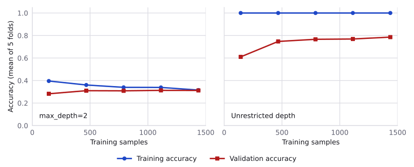
- High bias (
max_depth=2). The training accuracy falls and the validation accuracy rises until both are about 0.31. A tree of depth 2 has at most 4 leaves and therefore predicts at most 4 of the 10 digits. - High variance (unrestricted depth). The training accuracy is 1.000 at every size. The gap to the validation accuracy shrinks from 0.390 to 0.214, and the validation accuracy is still rising at the largest size.
More data therefore helps a model with high variance, but not one whose curves have already converged.
Remedies
Training and validation scores, with a learning curve where needed, identify the failure. A remedy for one failure tends to worsen the other, so every change is checked on validation data.
| Symptom | Likely cause | Remedies |
|---|---|---|
| Training and validation scores both poor and close; more data does not help | High bias (underfitting) | More informative features; polynomial features; weaker regularisation; a more flexible model, such as gradient boosting |
| Training score much better than validation score; the gap shrinks with more data | High variance (overfitting) | More data; stronger regularisation (Ridge and Lasso, C); smaller trees; averaging many trees; early stopping; fewer features, selected on the training data only |
| Validation score much better than the hidden test score | Leakage, or overfitting to validation data | Preprocessing fitted on training data only; the safeguards in the next section |
Overfitting to validation data
Every validation score contains noise. When many candidates are compared on the same validation data and the best is kept, the choice favours candidates whose errors happened to be small on those samples. The best score therefore overstates performance on new data, and the overstatement grows with the number of comparisons: the selection has overfitted the validation data. Hyperparameter Tuning measures the effect. A public leaderboard is such a validation set; in the IOAI 2026 Individual Contest, the live leaderboard and the final ranking use different hidden sets, as the note on local test sets describes.
The safeguards are a test set used once, at the end; cross-validation instead of one split; and treating differences within the noise of the validation set as ties.
Resources
| Source | Title | Why read it |
|---|---|---|
| scikit-learn | User Guide: Validation curves: plotting scores to evaluate models | The sections “Validation curve” and “Learning curve” describe validation_curve and learning_curve and how to read their plots. |
| scikit-learn | Underfitting vs. Overfitting | Polynomials of degree 1, 4 and 15 fitted to noisy samples of a cosine, compared by cross-validated error. |
| Google for Developers | Overfitting | The sections “Detecting overfitting” and “What causes overfitting?” cover loss curves, generalisation curves and the two main causes of overfitting. |
| Google for Developers | Overfitting: Interpreting loss curves | Four exercises on reading loss curves, including one in which the test loss diverges from the training loss. |
| James et al. | An Introduction to Statistical Learning with Python, section 2.2.2 | Free book. Section 2.2.2, “The Bias-Variance Trade-Off”, states the same decomposition without proof and plots squared bias, variance and test MSE for three examples in Figure 2.12. |
| StatQuest | Machine Learning Fundamentals: Bias and Variance | Bias, variance and overfitting defined on one small example. The video description corrects the statement at 4:06: variance is the amount by which predictions change when the model is fitted to a different training set. |