4Classical Machine Learning 4.3Classical Machine Learning Models
4.3.1Linear Regression
Predict a number from one or more features, measure the model's mistakes, and improve it with feature engineering.
What linear regression does
Linear regression is the most basic model of all models in Classical ML. It basically sets the precedent for what a model does, and how we basically build models. Linear regression predicts a number from one or more features. For example, it can use a flower's petal length to predict its petal width, or use a house's area, age and location to predict its price.
Its central idea is simple: give each feature a weight, add the weighted values, then add a constant. With one feature , the prediction is
Here:
- is the predicted value;
- is the feature's weight, also called the slope; and
- is the intercept, also called the bias.
Because this expression draws a straight line, the one-feature version is called simple linear regression. It basically figures out the pattern in the data that is given to it. The model is quick to train, easy to inspect and a useful baseline whenever the label is numeric. A more complicated model is worth using only if it can improve on that baseline.
Linear regression also introduces ideas that appear throughout machine learning: measuring errors with a loss, learning parameters that reduce that loss, and checking performance on unseen data. Logistic regression begins with the same weighted sum and turns it into a probability, while neural networks combine many weighted sums.
If some of the words or symbols here are unfamiliar, Terminology introduces the dataset notation, and NumPy Basics covers the array operations used in the examples.
One feature: fitting a line
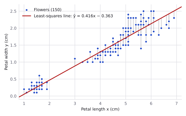
Consider the Iris dataset. This dataset is the dataset we will be using throughout this module to demonstrate how the linear regression model works. The datasets covers 150 iris flowers and tracks their physical traits and values along with their species. For each of its 150 flowers, suppose we use petal length to predict petal width. Both are measured in centimetres. Three rows look like this:
| Flower | Petal length (cm) | Petal width (cm) |
|---|---|---|
| 1 | 1.4 | 0.2 |
| 51 | 4.7 | 1.4 |
| 101 | 6.0 | 2.5 |
Longer petals tend to be wider, so a rising line seems reasonable. However, different choices of and give different lines. We need a consistent way to decide which one fits the data best.
From individual errors to one loss
For flower , the difference between its true width and its predicted width is called the residual:
A residual of means the prediction is exact. A positive residual means the prediction was too low, and a negative one means it was too high.
One residual describes one prediction. To judge the whole line, we combine all residuals into one number. Linear regression normally uses the mean squared error (MSE):
Squaring prevents positive and negative residuals from cancelling each other out. It also makes one large error count more heavily than several small errors. Training linear regression means finding the weights and intercept that make this loss as small as possible. This approach is also called least squares.
You may also see the sum of squared residuals,
MSE is simply , so both are smallest for the same line. The squared loss is also smooth, which lets calculus find its minimum.
Finding the best line
With one feature, the best slope and intercept can be calculated directly. If is the mean feature value and is the mean label, then
The numerator in the formula for is positive when and tend to rise together. The formula for makes the fitted line pass through the point .
OptionalOptional mathematics: where the formulas come from
At the minimum, changing either or by a tiny amount cannot reduce SSR further, so both derivatives are zero. The derivative with respect to gives
Substituting this result into SSR and setting the derivative with respect to to zero gives the slope formula above. This is the one-feature version of the normal equation introduced later.
Here is the calculation for the Iris petals, followed by the same fit in scikit-learn:
import numpy as np
from sklearn.datasets import load_iris
from sklearn.linear_model import LinearRegression

iris = load_iris()
length = iris.data[:, 2]  # petal length (cm), the feature
width = iris.data[:, 3]   # petal width (cm), the target

x_mean, y_mean = length.mean(), width.mean()
dx, dy = length - x_mean, width - y_mean
w = np.sum(dx * dy) / np.sum(dx ** 2)
b = y_mean - w * x_mean
print(round(w, 4), round(b, 4))
# 0.4158 -0.3631

model = LinearRegression()
model.fit(length.reshape(-1, 1), width)
print(round(model.coef_[0], 4), round(model.intercept_, 4))
# 0.4158 -0.3631
Both methods find the same line:
The slope says that adding 1 cm to petal length adds about 0.416 cm to the predicted petal width. For a petal length of 4.0 cm, the predicted width is cm. The MSE on the 150 training flowers is 0.0421.
Several features: the same idea, repeated
Real problems usually provide more than one useful feature. With features, each one receives its own weight:
The expression is the dot product: multiply each feature by its matching weight and add the results. In NumPy, it is written w @ x. With two features, the model describes a plane instead of a line. With more features, the same calculation continues even though we can no longer draw it easily.
The diabetes dataset in scikit-learn contains ten measurements for each of 442 patients. Its numeric label measures disease progression one year later. A model using age, body mass index (BMI) and average blood pressure works like this:
from sklearn.datasets import load_diabetes

diabetes = load_diabetes(scaled=False, as_frame=True)
X3 = diabetes.data[["age", "bmi", "bp"]].to_numpy()
y_all = diabetes.target.to_numpy()

model3 = LinearRegression().fit(X3, y_all)
w3, b3 = model3.coef_, model3.intercept_
print(w3.round(3), round(b3, 2))
# [0.094 8.502 1.357] -205.11

x_1 = X3[0]  # age 59, BMI 32.1, blood pressure 101
print(round(w3 @ x_1 + b3, 2))
print(model3.predict(X3[:1]).round(2))
# 210.41
# [210.41]
For this patient, the calculation is
That is exactly what predict does. A linear model is still just a weighted sum, no matter how many features it receives.
Using LinearRegression in practice
The usual workflow is short: split the data, fit on the training part, and predict the part the model did not see.
from sklearn.model_selection import train_test_split

X = diabetes.data.to_numpy()
y = diabetes.target.to_numpy()

X_train, X_test, y_train, y_test = train_test_split(
    X, y, test_size=0.2, random_state=0
)

model = LinearRegression()
model.fit(X_train, y_train)
y_pred = model.predict(X_test)

print(model.coef_)      # one learned weight per feature
print(model.intercept_) # the learned constant
fit learns the weights and intercept from X_train and y_train. predict uses those learned values for new rows. The fitted values are available as coef_ and intercept_.
LinearRegression also has a fit_intercept option, which is True by default. Setting it to False forces , so the fitted line or plane must pass through the origin. Its positive option is False by default; setting it to True forces every weight to be non-negative.
Evaluating predictions on unseen data
Now that the model has made predictions for X_test, we can judge how well it generalises. Three common regression metrics are:
- MSE: the average squared error. Smaller is better.
- RMSE: the square root of MSE. It is useful because it has the same units as the label.
- : a comparison with always predicting the mean label. A score of 1 is perfect, 0 is about as useful as the mean, and a score can be negative on unseen data.
from sklearn.metrics import mean_squared_error, r2_score

mse = mean_squared_error(y_test, y_pred)
rmse = np.sqrt(mse)
r2 = r2_score(y_test, y_pred)

print(round(mse, 1), round(rmse, 1), round(r2, 3))
# 3424.3 58.5 0.332
On these held-out patients, the model's RMSE is 58.5 progression units and its is 0.332. In other words, its predictions are off by 58.5 units in the root-mean-square sense, and it explains about a third of the variation in the unseen labels. Model Evaluation Metrics compares these with other choices, such as mean absolute error.
Interpreting the weights
A weight answers this question:
If feature increases by one unit while the other features stay fixed, how much does the prediction change?
That last condition matters. The weights describe the model, not necessarily cause and effect in the real world.
The unit also matters. If we measure Iris petal length in millimetres instead of centimetres, the values become ten times larger. The weight becomes ten times smaller, but every prediction stays the same:
model_mm = LinearRegression().fit(10 * length.reshape(-1, 1), width)
print(round(model_mm.coef_[0], 4), round(model_mm.intercept_, 4))
# 0.0416 -0.3631
This is why raw coefficient sizes should not be used to compare features measured on different scales. On the ten diabetes features in their original units, the weight for BMI is 5.603 and the weight for s5 is 68.483. However, BMI has a standard deviation of 4.41 while s5 has a standard deviation of 0.52, so a one-unit change means something very different for each. After standardisation, the weights are 24.7 for BMI and 35.7 for s5, making their scales more comparable.
Even then, correlated features can make individual weights unstable. We will see that limitation next.
Where a straight-line model can fail
Linear regression is a useful baseline, not a universal answer. Four problems appear often.
Outliers
Because MSE squares every residual, one extreme error can strongly pull the fitted line. If one Iris petal width is changed from 0.2 cm to 20 cm, the line moves from to . Loss Functions describes losses that are less sensitive to outliers.
Extrapolation
A fitted line continues forever, even when its predictions stop making sense. The Iris model's intercept is , its prediction at a petal length of 0. At 0.5 cm it predicts a width of cm. No flower in the training data has petals shorter than 1.0 cm, so this is a warning against trusting the model outside the range it has seen.
Non-linear relationships
Some relationships are curved, so a straight line is simply the wrong shape. A regular pattern in the residuals, such as positive residuals at both ends and negative residuals in the middle, is a useful clue that the model is missing curvature.
Correlated features
Two features can carry nearly the same information. In the diabetes data, s1 and s2 have a correlation of 0.897. Removing s2 changes the weight of s1 from to and the weight of s5 from 68.483 to 48.869, while the training falls only from 0.5177 to 0.5155. The predictions barely change, but the individual weights do, so correlated coefficients should not be interpreted one at a time.
Fitting curves by creating better features
"Linear" means that the prediction is linear in the learned weights. The input features themselves do not have to be straight or simple. If the original features are and , we can create
and fit a weighted sum of all five. This is still linear regression, but it can now describe quadratic relationships. Scikit-learn's PolynomialFeatures creates these columns:
from sklearn.preprocessing import PolynomialFeatures

ab = np.array([[2.0, 3.0], [1.0, 0.0], [-1.0, 2.0]])
poly = PolynomialFeatures(degree=2, include_bias=False)
expanded = poly.fit_transform(ab)

print(poly.get_feature_names_out(["a", "b"]))
# ['a' 'b' 'a^2' 'a b' 'b^2']
print(expanded)
# [[ 2.  3.  4.  6.  9.]
#  [ 1.  0.  1.  0.  0.]
#  [-1.  2.  1. -2.  4.]]
For a real example, consider the mean radius and mean area of cell nuclei in the Breast Cancer dataset. Area grows roughly with the square of radius. A straight line misses that curve, while adding radius squared captures it:
from sklearn.datasets import load_breast_cancer
from sklearn.metrics import root_mean_squared_error
from sklearn.pipeline import make_pipeline

cancer = load_breast_cancer(as_frame=True)
radius = cancer.data[["mean radius"]]
area = cancer.data["mean area"]
r_train, r_test, a_train, a_test = train_test_split(
    radius, area, test_size=0.2, random_state=0
)

for degree in [1, 2]:
    curved_model = make_pipeline(
        PolynomialFeatures(degree, include_bias=False),
        LinearRegression(),
    )
    curved_model.fit(r_train, a_train)
    pred = curved_model.predict(r_test)
    rmse = root_mean_squared_error(a_test, pred)
    print(degree, round(rmse, 1), curved_model[-1].coef_.round(2))
# 1 50.2 [100.]
# 2 12.5 [0.02 3.12]
The quadratic features lower the test RMSE from 50.2 to 12.5. The weight of radius squared is 3.12, close to , as we would expect from the area of a circle.
The residuals tell the same story. For the straight-line model's training predictions, the mean residual is for the 32 tumours with radius below 10, for the 389 between 10 and 20, and for the 34 above 20. This regular positive-negative-positive pattern is a sign that a curved term is missing.
The general lesson is important: feature engineering changes the relationships a linear model can represent.
More features can lead to overfitting
Polynomial features are powerful, but their number grows quickly. Degree-3 polynomial expansion turns the ten diabetes features into 285 columns. That is a lot of flexibility for only 353 training patients.
ols = make_pipeline(
    PolynomialFeatures(degree=3, include_bias=False),
    LinearRegression(),
).fit(X_train, y_train)

print(ols[0].n_output_features_)  # 285
print(round(ols.score(X_train, y_train), 3))  # 0.887
print(round(ols.score(X_test, y_test), 3))    # -5.627
The model achieves on the training data but on the test data. The exact scores can vary with the numerical solver version because many expanded columns are nearly redundant, but the conclusion is unchanged: the test score is extremely poor. The model has learned details of the training set that do not carry over to new patients. This is overfitting.
Methods for controlling overfitting belong to the Silver-level material. For now, the important lesson is to compare training and unseen-data scores whenever feature engineering makes the model more flexible.
How the model learns its weights
You can use linear regression without knowing its solver. Scikit-learn's LinearRegression solves the least-squares problem directly. The main idea behind that calculation is described below.
Direct solution with a design matrix
For all samples at once, place the feature rows in a matrix . Add a column of ones for the intercept to form the design matrix , and collect the parameters into . All predictions are then
Least squares chooses to minimise , the sum of squared residuals.
OptionalOptional mathematics: the normal equation and SVD
Setting the gradient of the squared error to zero gives the normal equation
If the columns of are independent, this is sometimes written as
This formula is useful for understanding the result, but code should not calculate the inverse explicitly. Libraries use more stable numerical methods.
A = np.column_stack([np.ones(len(X)), X])

theta_ne = np.linalg.solve(A.T @ A, A.T @ y)
theta_ls = np.linalg.lstsq(A, y)[0]

lin = LinearRegression().fit(X, y)
theta_sk = np.concatenate([[lin.intercept_], lin.coef_])
print(np.allclose(theta_ne, theta_sk), np.allclose(theta_ls, theta_sk))
# True True
A problem appears when one feature is a weighted copy of other features. For example, petal length in millimetres is exactly ten times petal length in centimetres. Adding both gives no new information, so many different pairs of weights make the same predictions.
A2 = np.column_stack([np.ones(150), length, 10 * length])
print(np.linalg.matrix_rank(A2))  # 2, although A2 has 3 columns

theta_inv = np.linalg.inv(A2.T @ A2) @ A2.T @ width
theta_lst = np.linalg.lstsq(A2, width)[0]
for theta in [theta_inv, theta_lst]:
    duplicate_mse = np.mean((A2 @ theta - width) ** 2)
    print(theta.round(4), round(duplicate_mse, 4))
# [0.513  0.0661 0.0164] 0.1807
# [-0.3631  0.0041 0.0412] 0.0421
Mathematically, has no inverse here. Floating-point rounding can make it appear invertible, but the direct inverse magnifies tiny rounding errors and returns a poor answer. lstsq still returns a valid least-squares solution.
Scikit-learn handles this with the singular value decomposition (SVD). SVD writes as and uses those simpler matrices to solve least squares without forming . This stays accurate when features are nearly redundant. For , the computation costs about .
Section 1.2 of the CS229 lecture notes derives the normal equation step by step.
What about gradient descent?
Gradient descent is another way to learn a model's weights. It will be discussed in Gradient Descent in the deep-learning section.
Optional: linear regression from scratch
This function builds the design matrix and passes it to NumPy's least-squares solver:
def fit_lstsq(X, y):
    A = np.column_stack([np.ones(len(X)), X])
    theta = np.linalg.lstsq(A, y)[0]
    return theta[1:], theta[0]


sk = LinearRegression().fit(X, y)
w_ls, b_ls = fit_lstsq(X, y)

print(sk.coef_[:4].round(3), round(sk.intercept_, 3))
print(w_ls[:4].round(3), round(b_ls, 3))
# [ -0.036 -22.86    5.603   1.117] -334.567  (both lines)
print(np.allclose(w_ls, sk.coef_))  # True
The NumPy implementation reproduces scikit-learn's result.
Linear regression in olympiad tasks
Because the model was fixed, progress came from better features. Linear regression can add its input features with different weights, but it cannot square, multiply or compare them unless those operations have already been turned into features.
The baseline used the first 300 raw values of each array—only the first two of five slices along one axis—and received a validation score of 6.818. The organisers' reference solution then:
- used the arrays' symmetries to enlarge the training set with permuted spatial axes;
- compressed the arrays to 299 components with principal component analysis; and
- added one hand-designed feature from the preceding at-home task.
The first two changes lowered the score to 3.707. Adding the hand-designed feature lowered it again to 1.651. The lesson is broader than this task: a simple model with excellent features can outperform a more sophisticated-looking pipeline with poor features.
The whole idea in one view
Linear regression can be remembered as four connected loops:
prediction:      features → weighted sum → predicted number
training:        predictions → residuals → MSE → learn weights
generalisation:  train on one part → evaluate on unseen data
improvement:     curved pattern → new features
                 too many features → check performance on unseen data
Start with LinearRegression, measure its performance on unseen data, and inspect where it goes wrong. Those mistakes tell you whether the next step should be better features, a more suitable loss, or a different model.
Resources
| Source | Title | Why read it |
|---|---|---|
| scikit-learn | User Guide: Linear Models | The section 'Ordinary Least Squares' explains the objective used by LinearRegression. |
| Google for Developers | Linear regression | The sections 'Linear regression equation' and 'Models with multiple features' introduce the model with a worked example. |
| Google for Developers | Linear regression: Loss | Compares squared and absolute loss and how each reacts to outliers. |
| Stanford CS229 (Tengyu Ma and Andrew Ng) | CS229 Lecture Notes, chapter 1: Linear regression | Section 1.2 derives the normal equations, and section 1.3 shows least squares as maximum likelihood. |
| James, Witten, Hastie, Tibshirani | An Introduction to Statistical Learning | A free textbook whose regression chapter covers this module's material with more statistical depth. |
Practice problems
| Solved | Source | Problem | Difficulty | Tags |
|---|---|---|---|---|
| Kaggle | House Prices | Medium | regression, feature engineering | |
| IOAI 2024 | Lost in Hyperspace | Hard | regression, feature engineering |