4Classical Machine Learning 4.3Classical Machine Learning Models
4.3.2Logistic Regression
Classification with a linear model: the sigmoid function, log-odds, log loss, regularisation, multi-class extensions and use in scikit-learn.
Many tasks ask not for a number but for a category. Is this tumour malignant or benign? Was this sentence written by a person or generated by a language model? Which of six actions will a robot take next? These are classification problems, and they are at least as common in contests as predicting numbers.
Logistic regression is the simplest model for such questions, and it answers with a probability for each category rather than only a guess. That matters in practice: a probability shows how confident the model is, lets you move the decision threshold when one kind of mistake is worse than the other, and is exactly what metrics such as ROC AUC and log loss need.
It is the classification counterpart of linear regression, so most of what you learned there carries over. It also works well on features produced by a pretrained network: the IOAI 2026 hints for Ghost of the Machine suggest exactly this, a logistic regression trained on sentence embeddings.
Logistic regression is a model for classification. Despite its name, it does not predict a real-valued label: it passes the weighted sum of linear regression through a function that turns it into a probability, and assigns the class with the higher probability. It is fast, it has a convex training objective with a single minimum, its weights can be interpreted, and it is one of the strongest baselines for classification on tabular data and on precomputed features.
Why not linear regression?
The Breast Cancer dataset in scikit-learn describes 569 tumours by 30 numeric features computed from images of cell nuclei. In this module the label is for a malignant tumour (212 samples) and for a benign one (357 samples); scikit-learn stores the opposite coding, so the target is converted first.
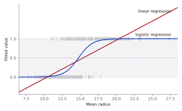
Linear regression can be fitted to 0/1 labels, and its prediction can be compared with 0.5 to assign a class. On one feature, the mean radius of the nuclei, this already exposes two problems.
import numpy as np
import pandas as pd
from sklearn.datasets import load_breast_cancer
from sklearn.linear_model import LinearRegression

data = load_breast_cancer(as_frame=True)
X = data.data
y = (data.target == 0).astype(int)  # 1 = malignant, 0 = benign
print(X.shape, y.sum())             # (569, 30) 212

radius = X[["mean radius"]]
lin = LinearRegression().fit(radius, y)
y_lin = lin.predict(radius)
print(round(y_lin.min(), 2), round(y_lin.max(), 2))  # -0.34 1.77
print((y_lin < 0).sum(), (y_lin > 1).sum()) # 60 35- The outputs are not probabilities. The fitted values range from to : 60 tumours receive a value below 0 and 35 a value above 1.
- Correct, confident predictions distort the fit. The largest tumour, with mean radius 28.11, is malignant, and the line predicts 1.774 for it. Squared error penalises this correct prediction by , and such points pull the line and move the 0.5 threshold.
far = X["mean radius"] > 18          # 92 tumours, all malignant
lin_near = LinearRegression().fit(radius[~far], y[~far])
for model in (lin, lin_near):
    # the radius at which the fitted line equals 0.5
    print(round((0.5 - model.intercept_) / model.coef_[0], 2))
# 15.4
# 15.01
All 92 tumours with a mean radius above 18 are malignant, and both lines classify them correctly. Yet removing them moves the linear threshold from 15.40 to 15.01. For the logistic regression fitted below, the corresponding boundary moves only from 14.75 to 14.79.
The sigmoid function
Its values for a few inputs show its shape:
| 0.0025 | 0.0180 | 0.1192 | 0.2689 | 0.5 | 0.7311 | 0.8808 | 0.9820 | 0.9975 |
- . Large positive gives values close to 1, and large negative values close to 0.
- The function is symmetric about this point: .
- Its derivative has the convenient form , which is largest, 0.25, at . This form makes the gradient of the training loss simple.
This function has exactly the properties we wanted. But where does it come from? One way to arrive at it is to ask for a curve whose rate of change is proportional to both its current value and the space left before it reaches 1:
When is close to 0 or 1, the product is small, so the curve flattens. It changes fastest halfway between them. The nonconstant solutions to this differential equation form a family of logistic curves,
Requiring gives , leaving exactly the sigmoid function. This is one mathematical route to the curve, rather than something you need to derive whenever you use logistic regression. If you want to see the calculus in full, Khan Academy's Logistic models with differential equations works through it. The log-odds interpretation below gives the reason this same curve fits naturally into a classifier.
The model
Odds and log-odds
The odds of an event with probability are : a probability of 0.8 corresponds to odds of 4, or "4 to 1", and a probability of 0.5 to odds of 1. Solving for gives
so the model is linear in the log-odds. This fixes the meaning of a weight: increasing feature by one unit, with the other features fixed, adds to the log-odds and therefore multiplies the odds by .
from sklearn.linear_model import LogisticRegression

log_reg = LogisticRegression(C=np.inf)  # no regularisation
log_reg.fit(radius, y)
w = log_reg.coef_[0, 0]
b = log_reg.intercept_[0]
print(round(w, 3), round(b, 2))  # 1.034 -15.25
print(round(np.exp(w), 2))       # 2.81: odds ratio for +1 in radius

new = pd.DataFrame({"mean radius": [14.0, 15.0, 16.0]})
p = log_reg.predict_proba(new)[:, 1]
print(p.round(3))                # [0.315 0.564 0.785]
print((p / (1 - p)).round(3))    # [0.46  1.295 3.641]: odds
print(round(-b / w, 2))          # 14.75: decision boundary
Each additional unit of mean radius multiplies the odds of malignancy by : from 0.460 to 1.295 to 3.641. The probability does not change by a constant amount: it rises by 0.249 from radius 14 to 15 and by 0.220 from 15 to 16, because the sigmoid flattens as it approaches 1.
Weights can be interpreted one at a time only when features are not strongly correlated. Mean radius has a correlation of 0.9979 with mean perimeter and 0.9874 with mean area, so in a model with all three the credit is shared among them in ways that change from one fit to the next.
The decision boundary
The model predicts class 1 when . Since exactly at , this is the same as . The set of points where is the decision boundary: a single threshold for one feature (a mean radius of 14.75 above), a straight line for two features, and a flat surface called a hyperplane in general. Logistic regression is therefore a linear classifier.
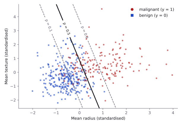
The threshold 0.5 is a convention, not a requirement. When one kind of error is more costly than the other, such as missing a malignant tumour, a lower threshold on trades more false alarms for fewer misses. Model Evaluation Metrics describes how to choose it.
Training with log loss
Logistic regression is trained by choosing the and under which the observed labels are as probable as possible. For three samples with labels and predicted probabilities of class 1 of , the model assigns the observed labels the probabilities , and . Assuming independent samples, the probability of all three, the likelihood, is .
Maximising a product is awkward, so the logarithm is taken, which turns it into a sum, and the sign is flipped to obtain a quantity to minimise. Divided by , this is the log loss.
from sklearn.metrics import log_loss

y_true = [1, 0, 1]
p_hat = [0.9, 0.2, 0.6]
by_hand = -np.mean(np.log([0.9, 1 - 0.2, 0.6]))
print(round(by_hand, 4), round(log_loss(y_true, p_hat), 4))
# 0.2798 0.2798
The loss of a single sample with label 1 grows quickly as its predicted probability falls:
| for a sample with | 0.99 | 0.9 | 0.5 | 0.1 | 0.01 |
|---|---|---|---|---|---|
| Loss | 0.010 | 0.105 | 0.693 | 2.303 | 4.605 |
A confident correct prediction costs almost nothing, and a confident wrong prediction costs a lot, which is the behaviour a classifier should be trained towards. Loss Functions compares log loss with the other common losses.
The gradient
With and , the derivative of one sample's loss with respect to its score simplifies, using , to
By the chain rule, since and ,
The gradient has the same form as for linear regression: the error , weighted by the features. In matrix form, .
Unlike least squares, setting this gradient to zero has no closed-form solution, so the minimum is found iteratively. The log loss of logistic regression is convex: it has no local minima other than the global one, so gradient descent with a suitable learning rate reaches the best parameters from any starting point.
function gradient_descent(X, y, learning_rate, n_iter):
    n, d = shape of X
    w = zeros(d)
    b = 0
    repeat n_iter times:         # or until the loss stops decreasing
        p_hat = sigmoid(X @ w + b)   # probabilities of class 1
        grad_w = (1 / n) * X.T @ (p_hat - y)
        grad_b = (1 / n) * sum(p_hat - y)
        w = w - learning_rate * grad_w   # learning_rate is η
        b = b - learning_rate * grad_b
return w, bRegularisation
When the classes can be separated perfectly by a hyperplane, the log loss has no minimum at finite weights. Multiplying all weights of a separating model by 2, 4 or 8 pushes every probability closer to the correct 0 or 1 and keeps lowering the loss. On the task of separating setosa from the other two Iris species, which is perfectly separable, the loss falls from 0.017 to as the weights are scaled from 1 to 8 times their fitted size. Without regularisation, the weights grow without bound. Even without perfect separation, large weights produce overconfident probabilities that overfit.
Scikit-learn therefore adds an L2 penalty by default, the same kind of penalty as Ridge regression. Its objective is equivalent to
where is the log loss of sample , and is the inverse of the regularisation strength: a smaller means a stronger penalty and smaller weights. The following code fits standardised models with different values of on a stratified 80/20 split.
from sklearn.model_selection import train_test_split
from sklearn.pipeline import make_pipeline
from sklearn.preprocessing import StandardScaler

X_train, X_test, y_train, y_test = train_test_split(
    X, y, test_size=0.2, stratify=y, random_state=0
)
for C in [0.001, 0.01, 0.1, 1, 10, 100, 1000]:
    m = make_pipeline(StandardScaler(), LogisticRegression(C=C))
    m.fit(X_train, y_train)
    norm = np.linalg.norm(m[-1].coef_)
    train_acc = m.score(X_train, y_train)
    test_acc = m.score(X_test, y_test)
print(C, round(norm, 2), round(train_acc, 3), round(test_acc, 3))| Size of the weights | Training accuracy | Test accuracy | |
|---|---|---|---|
| 0.001 | 0.30 | 0.897 | 0.921 |
| 0.01 | 0.84 | 0.954 | 0.965 |
| 0.1 | 1.83 | 0.987 | 0.974 |
| 1 | 3.65 | 0.993 | 0.974 |
| 10 | 8.50 | 0.993 | 0.965 |
| 100 | 25.17 | 0.996 | 0.947 |
| 1000 | 65.49 | 1.000 | 0.947 |
As grows, the weights grow and the training accuracy rises to 1.000, while the test accuracy peaks at and and then falls: very small underfits and very large overfits. is a hyperparameter to be chosen by cross-validation.
An L1 penalty, as in Lasso, sets some weights exactly to zero. In scikit-learn 1.9.1 it is selected with l1_ratio=1 (the default l1_ratio=0 is the L2 penalty). The older penalty parameter is deprecated since version 1.8. The default solver, "lbfgs", supports only the L2 penalty, so the L1 penalty needs a solver such as "liblinear":
sparse = make_pipeline(
    StandardScaler(),
    LogisticRegression(C=0.1, l1_ratio=1, solver="liblinear",
                       random_state=0),
)
sparse.fit(X_train, y_train)
print((sparse[-1].coef_ != 0).sum())  # 7 non-zero weights out of 30
Feature scaling and convergence
Scikit-learn minimises the objective with an iterative solver that stops after max_iter iterations, 100 by default. On unscaled features the problem is badly conditioned: the breast cancer features range from 0.05 to 0.16 for mean smoothness and from 143.5 to 2,501 for mean area.
raw = LogisticRegression().fit(X_train, y_train)
print(raw.n_iter_)    # [100]  (with a ConvergenceWarning)

model = make_pipeline(StandardScaler(), LogisticRegression())
model.fit(X_train, y_train)
print(model[-1].n_iter_)          # [18]
print(model.score(X_test, y_test))  # 0.9736842105263158
On the raw features, the solver reaches the limit and issues a ConvergenceWarning: lbfgs failed to converge after 100 iteration(s). Given enough iterations it needs 2,679 of them. On standardised features it converges in 18. Standardising the features, rather than raising max_iter, is the correct response to this warning, and it also makes the L2 penalty treat all features equally.
More than two classes
Multinomial logistic regression
For classes, the model has one weight vector and one intercept per class, and computes a score for each. The softmax function turns the scores into probabilities that are positive and sum to 1:
For , the softmax probability of one class equals the sigmoid of the difference of the two scores, so this model generalises the binary case. It is trained with the multi-class log loss, . With the default solver, scikit-learn 1.9.1 fits this multinomial model whenever there are three or more classes; the former multi_class parameter no longer exists.
from sklearn.datasets import load_iris

X_iris, y_iris = load_iris(return_X_y=True)
iris_model = make_pipeline(StandardScaler(), LogisticRegression())
iris_model.fit(X_iris, y_iris)
print(iris_model[-1].coef_.shape)  # (3, 4): a row per class

z = iris_model.decision_function(X_iris[:2])  # shape (2, 3)
p_softmax = np.exp(z) / np.exp(z).sum(axis=1, keepdims=True)
print(np.allclose(p_softmax, iris_model.predict_proba(X_iris[:2])))
# True
One-vs-rest
An alternative trains separate binary classifiers, each separating one class from all the others, and predicts the class whose classifier gives the highest score. This one-vs-rest scheme is available by wrapping any binary classifier in OneVsRestClassifier. The "liblinear" solver supports only this approach and raises an error for three or more classes unless it is wrapped.
from sklearn.datasets import load_wine
from sklearn.model_selection import cross_val_score
from sklearn.multiclass import OneVsRestClassifier

for load in (load_iris, load_wine):
    X_d, y_d = load(return_X_y=True)
    for est in (LogisticRegression(),
                OneVsRestClassifier(LogisticRegression())):
        pipe = make_pipeline(StandardScaler(), est)
        acc = cross_val_score(pipe, X_d, y_d, cv=5).mean()
        print(load.__name__, type(est).__name__, round(acc, 3))
# load_iris LogisticRegression 0.96
# load_iris OneVsRestClassifier 0.927
# load_wine LogisticRegression 0.983
# load_wine OneVsRestClassifier 0.989
Neither approach is better on every dataset. The multinomial model is the default and is usually the first choice, since it produces a single consistent set of probabilities.
In scikit-learn
A fitted binary model stores one row of weights, and its three prediction methods are consistent with the formulas above.
clf = model[-1]
print(clf.classes_, clf.coef_.shape, clf.intercept_.shape)
# [0 1] (1, 30) (1,)

scores = model.decision_function(X_test)  # z for each sample
proba = model.predict_proba(X_test)       # shape (114, 2)
pred = model.predict(X_test)
print(scores[:3].round(2))  # [-7.89 -4.16 -1.23]
print(proba[:3].round(3))
# [[1.    0.   ]
#  [0.985 0.015]
#  [0.774 0.226]]

Z_test = model[:-1].transform(X_test)     # standardised features
print(np.allclose(scores, Z_test @ clf.coef_[0] + clf.intercept_))
print(np.allclose(proba[:, 1], 1 / (1 + np.exp(-scores))))
print(np.array_equal(pred, (scores > 0).astype(int)))
# True, True, True
decision_function returns , the second column of predict_proba is , and predict returns 1 exactly where .
| Parameter | Default | Meaning |
|---|---|---|
C |
1.0 |
Inverse of the regularisation strength; smaller values regularise more |
l1_ratio |
0.0 |
Type of penalty: 0 is L2 and 1 is L1 |
solver |
"lbfgs" |
Optimisation algorithm; "liblinear" supports L1 for binary problems |
max_iter |
100 |
Maximum number of solver iterations |
tol |
0.0001 |
Tolerance of the stopping criterion |
class_weight |
None |
"balanced" weights classes inversely to their frequency |
fit_intercept |
True |
Whether to fit the intercept |
From scratch in NumPy
The algorithm above, with the L2 penalty written to match scikit-learn's , fits in a few lines.
def sigmoid(z):
    return 1 / (1 + np.exp(-z))


def fit_logistic(X, y, C=1.0, lr=0.5, n_iter=10_000):
    n, d = X.shape
    lam = 1 / (n * C)  # L2 strength that matches scikit-learn's C
    w, b = np.zeros(d), 0.0
    for _ in range(n_iter):
        p = sigmoid(X @ w + b)
        grad_w = X.T @ (p - y) / n + lam * w
        grad_b = np.mean(p - y)
        w -= lr * grad_w
        b -= lr * grad_b
    return w, b


scaler = StandardScaler().fit(X_train)
Z_train, Z_test = scaler.transform(X_train), scaler.transform(X_test)
y_tr, y_te = y_train.to_numpy(), y_test.to_numpy()

w, b = fit_logistic(Z_train, y_tr, C=1.0)
acc = np.mean((Z_test @ w + b > 0) == y_te)

sk = LogisticRegression(C=1.0, tol=1e-10, max_iter=10_000)
sk.fit(Z_train, y_tr)
print(acc, sk.score(Z_test, y_te))   # 0.9736842105263158 (both)
print(np.abs(w - sk.coef_[0]).max())  # about 1.2e-06
print(abs(b - sk.intercept_[0]))      # about 2.9e-07
After 10,000 iterations on the standardised breast cancer features, the NumPy weights agree with scikit-learn's to within about , and both models make the same test predictions. The penalty term in the gradient is the derivative of . For very large negative scores, np.exp(-z) overflows, near ; scipy.special.expit computes the sigmoid without this problem.
Where logistic regression fits
- As a baseline. A standardised logistic regression trains in milliseconds on tabular data and often comes close to more complex models. Its test accuracy of 0.974 on the breast cancer split above is a demanding reference for any other model.
- On top of precomputed features. When a pretrained network turns images, text or audio into embedding vectors, a logistic regression trained on those vectors is a fast classifier, often called a linear probe.
- Its limit. The decision boundary is linear. When the classes are separated by a curve, the model fails unless the features are transformed first.
from sklearn.datasets import make_circles
from sklearn.preprocessing import PolynomialFeatures

X_c, y_c = make_circles(
    n_samples=500, noise=0.1, factor=0.5, random_state=0
)
linear = LogisticRegression()
quadratic = make_pipeline(
    PolynomialFeatures(degree=2), StandardScaler(),
    LogisticRegression(),
)
for m in (linear, quadratic):
    print(round(cross_val_score(m, X_c, y_c, cv=5).mean(), 3))
# 0.444
# 0.988
The data consist of two noisy concentric circles, one per class. A straight line cannot separate them, and plain logistic regression scores 0.444, worse than guessing. With degree-2 polynomial features, the boundary becomes a curve in the original two features, and the accuracy rises to 0.988.
Resources
| Source | Title | Why read it |
|---|---|---|
| scikit-learn | User Guide: Logistic regression | The sections “Binary Case”, “Multinomial Case” and “Solvers” give the exact objective scikit-learn minimises and which solver supports which penalty. |
| scikit-learn | LogisticRegression | Every parameter with its default, including the deprecation of penalty in favour of l1_ratio. |
| Google for Developers | Logistic regression: Calculating a probability with the sigmoid function | “Transforming linear output using the sigmoid function” shows the step from a linear score to a probability. |
| Google for Developers | Logistic regression: Loss and regularization | “Log Loss” and “Regularization in logistic regression” explain why the loss is not squared error and why regularisation is needed. |
| Khan Academy | Logistic models with differential equations | An optional calculus-based route to the logistic function, including the differential equation it solves. |
| James, Witten, Hastie, Tibshirani | An Introduction to Statistical Learning | A free textbook. Its chapter on classification treats logistic regression with more statistical depth. |
Practice problems
| Solved | Source | Problem | Difficulty | Tags |
|---|---|---|---|---|
| Kaggle | Titanic | Easy | binary classification, tabular | |
| IOAI 2026 | Ghost of the Machine | Hard | nlp, embeddings |