4Classical Machine Learning 4.3Classical Machine Learning Models
4.3.4Decision Trees
Models that predict through a sequence of threshold tests on single features, grown greedily by the CART algorithm for classification and regression.
A decision tree works like a game of twenty questions. It asks a series of simple yes-or-no questions about the features, such as whether a petal is wider than 0.8 cm, and each answer narrows down the possibilities until it reaches a prediction. This is close to how a person might write rules by hand, which makes a tree easy to read, explain and check.
Trees are also practical. They need almost no data preparation: features on very different scales and relationships that are not straight lines cause them no trouble. That makes a shallow tree a fast and readable baseline for tabular data, and its printed rules often show which features matter.
A single tree is rarely the strongest model on its own, because small changes in the data can change it a lot. Its real importance lies in what comes next: Random Forests and XGBoost, two of the most successful models for tabular data, are both built from many trees. In Save the Factory (IOAI 2024), the organisers even fixed the tree, and the whole task was to engineer features that it could use.
A decision tree predicts the label of a sample by applying a sequence of tests of the form "is feature at most ?" until it reaches an answer. Trees are used for both classification and regression. This module describes the structure of a tree, the CART algorithm (Classification and Regression Trees) that grows it, the impurity measures that guide the algorithm and the hyperparameters that limit its size. The terms used below are defined in Terminology.
Structure of a decision tree
Each level of a tree at most doubles the number of nodes, so a tree of depth has at most leaves and at most internal nodes. A tree of depth 1, with one test and two leaves, is called a decision stump.
The following code fits a tree of depth at most 2 to the Iris dataset and prints it with export_text.
from sklearn.datasets import load_iris
from sklearn.tree import DecisionTreeClassifier, export_text

iris = load_iris()
X, y = iris.data, iris.target

clf = DecisionTreeClassifier(max_depth=2, random_state=0)
clf.fit(X, y)
print(export_text(clf, feature_names=iris.feature_names))
|--- petal width (cm) <= 0.80
| |--- class: 0
|--- petal width (cm) > 0.80
| |--- petal width (cm) <= 1.75
| | |--- class: 1
| |--- petal width (cm) > 1.75
| | |--- class: 2Each line is a node, and the indentation shows its depth. The root tests petal width against 0.80 cm. Its left child is a leaf that predicts class 0 (setosa). Its right child tests petal width against 1.75 cm, and the two leaves below predict class 1 (versicolor) and class 2 (virginica). The tree uses only one of the four features and classifies 144 of the 150 flowers correctly.
Prediction
A sample is passed down from the root. At each internal node it moves to the left child if its value of the tested feature is at most the threshold, and to the right child otherwise. The prediction is the value stored in the leaf where it stops.
Sample 150 of Iris has petal width 1.8 cm. It fails the root test and moves right. It then fails and moves right again, to the leaf that predicts virginica, its true species.
x_new = X[149:150]                # sample 150: [5.9, 3.0, 5.1, 1.8]
print(clf.predict(x_new))                  # [2]
print(clf.predict_proba(x_new).round(3))   # [[0.    0.022 0.978]]
For a classification tree, predict_proba returns the class proportions among the training samples in the leaf. This leaf contains 1 versicolor and 45 virginica flowers, so the probabilities are and . A prediction needs one comparison per level, so its cost is proportional to the depth of the tree.
Regions of the feature space
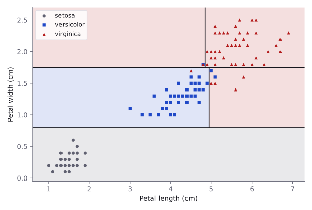
Each leaf corresponds to the samples that pass every test on its path. In the tree above, the middle leaf corresponds to . Such a set is a box whose sides are perpendicular to the feature axes, and the boxes of all leaves together cover the feature space without overlapping. A decision tree is therefore a piecewise constant function: it predicts a single value in each box.
Growing a tree
Finding the tree of a given size with the lowest training error is computationally hard. The scikit-learn User Guide notes that learning an optimal decision tree is NP-complete under several definitions of optimality, so no efficient exact algorithm is known. Practical algorithms therefore grow the tree greedily, one split at a time.
The depth-2 Iris tree above was grown in this way. CART first compared every split of the 150 flowers and chose petal width ≤ 0.80, which separates the 50 setosa flowers from the rest. It then repeated the search on each side. The left child was already pure and became a leaf; the right child, with the other 100 flowers, was split at petal width ≤ 1.75, and the depth limit of 2 then stopped the growth.
The scikit-learn User Guide also describes the older algorithms ID3 and C4.5. Unlike ID3, which builds a multiway tree, CART always makes binary splits; unlike C4.5, it supports numerical targets, that is, regression. DecisionTreeClassifier and DecisionTreeRegressor implement an optimised version of CART.
Notation
The right child of the root in the Iris tree provides a concrete case. It receives the 100 flowers that are not setosa: 50 versicolor and 50 virginica.
- denotes a node, and is the set of training samples that reach it. Here .
- A candidate split consists of a feature and a threshold . Here is petal width and .
- The split divides into , the samples with , and , the remaining samples. Here they contain and flowers.
- is the impurity of a set of samples: a number that is 0 when all labels in the set are equal and grows as the labels become more mixed. The next section defines it.
The quality of a split is the impurity of the two children, each weighted by its share of the samples:
CART chooses the split with the smallest weighted impurity. Equivalently, it maximises the impurity decrease , since does not depend on .
Candidate thresholds
In the training set, a feature takes finitely many values, so only finitely many splits are different. At each node, scikit-learn sorts the distinct values of feature among the samples there, , and tries the midpoints as thresholds.
At the root of the Iris tree, petal width has 22 distinct values, so 21 thresholds are tried for that feature. The largest petal width of a setosa is 0.6 cm, and the smallest of any other flower is 1.0 cm. The threshold 0.80 is the midpoint of these two consecutive values. Any threshold between 0.6 and 1.0 would divide the training data in the same way; the midpoint is the conventional choice.
function grow(samples, depth):
    if all labels in samples are equal or a stopping rule applies:
        # for example depth == max_depth; a leaf stores the class
        # proportions (classification) or the mean label (regression)
        return leaf(samples)

    best_split = none
    for each feature j:
        values = sorted distinct values of feature j in samples
        for each midpoint t between neighbouring values:
            G = weighted impurity of the split x[j] <= t
            if G is the smallest so far:
                best_split = (j, t)

    (j, t) = best_split
    left = samples with x[j] <= t
    right = all other samples
    return node(j, t, grow(left, depth + 1), grow(right, depth + 1))

tree = grow(all training samples, depth=0)
The algorithm is greedy: each split is the best one available at its node, regardless of the splits that could follow it. A split with a small impurity decrease that would enable very good splits below it can therefore be missed. The User Guide lists XOR and parity problems as concepts that trees do not express easily for this reason.
Impurity for classification
Both measures are 0 for a pure node, where one proportion equals 1, and both are largest when all classes are equally frequent. The Gini impurity is the probability that two samples drawn at random, with replacement, from the node have different labels. The entropy measures in bits the uncertainty about the label of a random sample from the node. For two classes, with a proportion of class 1:
| 0 | 0.1 | 0.25 | 0.5 | |
|---|---|---|---|---|
| Gini impurity | 0 | 0.18 | 0.375 | 0.5 |
| Entropy | 0 | 0.469 | 0.811 | 1 |
In scikit-learn, the criterion is chosen with criterion="gini" (the default) or criterion="entropy"; "log_loss" is a synonym for "entropy". The entropy uses base-2 logarithms: under criterion="entropy", the root of the Iris tree, with three equally frequent classes, has impurity .
Worked example: the second split of the Iris tree
The right child of the root splits on petal width at 1.75 cm. The class counts are:
| Node | Samples | Setosa | Versicolor | Virginica |
|---|---|---|---|---|
| Parent | 100 | 0 | 50 | 50 |
| Left child: petal width ≤ 1.75 | 54 | 0 | 49 | 5 |
| Right child: petal width > 1.75 | 46 | 0 | 1 | 45 |
- Parent. .
- Left child. .
- Right child. .
- Weighted impurity of the children. .
- Impurity decrease. .
No other feature or threshold at this node gives a smaller ; the best split on petal length, for comparison, reaches . The fitted tree stores the impurity of every node in clf.tree_.impurity, where the values 0.5, 0.168 and 0.0425 appear for these three nodes.
Regression trees
The mean is the constant with the smallest squared error. For a constant prediction , the sum of squared errors has derivative , which is zero exactly when . The impurity is the variance of the labels at the node, the error that remains after predicting the mean. Splits are chosen, as before, to minimise the weighted impurity of the children, so this criterion is also called variance reduction.
The diabetes dataset in scikit-learn records ten baseline variables for 442 patients. The label is a quantitative measure of disease progression one year after baseline. With scaled=False, the features keep their original units. The code fits a tree of depth 2 to a single feature, body mass index (BMI).
import numpy as np
from sklearn.datasets import load_diabetes
from sklearn.tree import DecisionTreeRegressor

diabetes = load_diabetes(scaled=False)
X_bmi = diabetes.data[:, [2]]     # one feature: body mass index
y_prog = diabetes.target          # disease progression after one year

reg = DecisionTreeRegressor(max_depth=2, random_state=0)
reg.fit(X_bmi, y_prog)
print(export_text(reg, feature_names=["bmi"]))

leaf = reg.apply(X_bmi)           # the leaf reached by each sample
for node in np.unique(leaf):
    in_leaf = leaf == node
    print(node, in_leaf.sum(), y_prog[in_leaf].mean().round(2))

print(reg.predict([[20.0], [24.0], [25.0], [30.0], [35.0]]).round(2))
|--- bmi <= 27.25
| |--- bmi <= 24.35
| | |--- value: [105.04]
| |--- bmi > 24.35
| | |--- value: [143.96]
|--- bmi > 27.25
| |--- bmi <= 33.15
| | |--- value: [191.56]
| |--- bmi > 33.15
| | |--- value: [264.23]
2 165 105.04
3 112 143.96
5 135 191.56
6 30 264.23
[105.04 105.04 143.96 191.56 264.23]The four leaves, nodes 2, 3, 5 and 6, hold 165, 112, 135 and 30 patients, and each stored value equals the mean label of its patients. As a function of BMI, the prediction is a step function with jumps at 24.35, 27.25 and 33.15. Every BMI up to 24.35 receives 105.04, and every BMI above 33.15 receives 264.23. A regression tree therefore never predicts outside the range of its leaf means, and the User Guide notes that trees are not good at extrapolation.
DecisionTreeRegressor also supports criterion="absolute_error", whose leaves predict the median, and criterion="poisson" for non-negative targets such as counts.
Overfitting and tree depth
Without limits, a tree keeps splitting until every leaf is pure or cannot be split further. It then fits the training labels almost perfectly, whether or not its splits reflect real structure. A training accuracy of 1 is therefore no evidence of a good tree. This is the overfitting described in Underfitting and Overfitting, and the depth of the tree is the most direct control over it.
The breast cancer dataset in scikit-learn contains 569 samples labelled malignant (212) or benign (357), each described by 30 numeric features computed from a digitised image of a breast mass. The code holds out 30% of the samples as a validation set and grows trees of increasing maximum depth.
from sklearn.datasets import load_breast_cancer
from sklearn.model_selection import train_test_split

cancer = load_breast_cancer()
X_train, X_val, y_train, y_val = train_test_split(
    cancer.data, cancer.target, test_size=0.3,
    stratify=cancer.target, random_state=0,
)
for depth in [1, 2, 3, 4, 5, 6, 8, None]:
    model = DecisionTreeClassifier(max_depth=depth, random_state=0)
    model.fit(X_train, y_train)
    train_acc = model.score(X_train, y_train)
    val_acc = model.score(X_val, y_val)
    print(depth, model.get_depth(), model.get_n_leaves(),
          f"{train_acc:.3f} {val_acc:.3f}")
max_depth |
Depth reached | Leaves | Training accuracy | Validation accuracy |
|---|---|---|---|---|
| 1 | 1 | 2 | 0.932 | 0.889 |
| 2 | 2 | 4 | 0.942 | 0.906 |
| 3 | 3 | 8 | 0.980 | 0.901 |
| 4 | 4 | 12 | 0.990 | 0.906 |
| 5 | 5 | 15 | 0.997 | 0.912 |
| 6 | 6 | 16 | 1.000 | 0.906 |
| 8 | 6 | 16 | 1.000 | 0.906 |
None |
6 | 16 | 1.000 | 0.906 |
- Training accuracy rises with depth and reaches 1.000 at depth 6, where every leaf is pure. The unrestricted tree also has depth 6, so every
max_depthof 6 or more produces the same tree. - Validation accuracy stays between 0.889 and 0.912 at every depth. The gap between training and validation accuracy grows from 0.043 at depth 1 to 0.094 for the full tree: the additional splits fit the training set without improving predictions on new data.
- One validation sample is worth of accuracy. Differences of one or two samples, such as the peak at depth 5, are not reliable. Cross-Validation gives steadier estimates for choosing the depth, as described in Hyperparameter Tuning.
Controlling the size of a tree
Limits applied while the tree grows are called pre-pruning. Scikit-learn also supports post-pruning, which grows a full tree and then removes its weakest branches, through the hyperparameter ccp_alpha, explained in the User Guide section “Minimal Cost-Complexity Pruning”. Scikit-learn provides the following, all of which apply to both DecisionTreeClassifier and DecisionTreeRegressor.
| Hyperparameter | Default | Effect |
|---|---|---|
max_depth |
None |
Largest depth of any leaf. With None, nodes are split until all leaves are pure or contain fewer than min_samples_split samples. |
min_samples_split |
2 |
A node with fewer samples is not split. A float is read as a fraction of the training samples. |
min_samples_leaf |
1 |
A split is considered only if it leaves at least this many training samples in each child. A float is read as a fraction. |
max_leaf_nodes |
None |
At most this many leaves. The tree is then grown best-first: nodes with the largest relative reduction in impurity are expanded first. |
min_impurity_decrease |
0.0 |
A node is split only if the weighted impurity decrease is at least this value. |
max_features |
None |
Number of features examined at each split, chosen at random. None examines all features and "sqrt" examines of the features. |
Setting max_features below the number of features makes each split examine a random subset of them. This rarely helps a single tree, but it is a key ingredient of Random Forests, which average many randomised trees. The User Guide suggests max_depth=3 as a starting depth for inspecting how a tree fits the data, and min_samples_leaf=5 as an initial value.
Properties of decision trees
No feature scaling
A split depends only on the order of a feature's values. A strictly increasing transformation of a feature, such as standardisation or for non-negative values, preserves that order. The tree then divides the training samples in the same way, and only the thresholds change. On the breast cancer split, trees fitted to the raw features, to standardised features and to of the features make identical predictions for all 171 validation samples. Distance-based models such as K-NN require scaling; trees do not.
Non-linear relationships and interactions
A tree assumes no functional form for the relationship between features and label. A regression tree approximates a curved relationship by steps, as in the BMI example. The tests along a path can involve several features, so a prediction can depend on a combination of them. In the depth-3 tree of the figure, a flower with petal width between 0.80 and 1.75 cm is predicted versicolor only if its petal length is at most 4.95 cm. The effect of petal length depends on petal width, which is called an interaction. Linear regression and logistic regression capture such an effect only if a feature representing it, such as a product of two features, is added by hand.
Axis-aligned boundaries
Each test involves a single feature, so every boundary between regions is parallel to a feature axis. A boundary in any other direction must be approximated by a staircase of small boxes. In the following example, two features are drawn uniformly from , and a sample belongs to class 1 exactly when , so the true boundary is the diagonal.
rng = np.random.default_rng(0)
P = rng.uniform(size=(2000, 2))            # two features in [0, 1]
labels = (P[:, 0] > P[:, 1]).astype(int)   # 1 below the diagonal
P_train, P_test, l_train, l_test = train_test_split(
    P, labels, test_size=0.5, random_state=0
)
for depth in [1, 2, 4, 8]:
    model = DecisionTreeClassifier(max_depth=depth, random_state=0)
    model.fit(P_train, l_train)
    print(depth, model.get_n_leaves(),
          round(model.score(P_test, l_test), 3))

D_train = (P_train[:, 0] - P_train[:, 1]).reshape(-1, 1)
D_test = (P_test[:, 0] - P_test[:, 1]).reshape(-1, 1)
stump = DecisionTreeClassifier(max_depth=1, random_state=0)
stump.fit(D_train, l_train)
print(stump.score(D_test, l_test))         # 1.0
1 2 0.729
2 4 0.857
4 13 0.951
8 30 0.976With 30 leaves, the tree still misclassifies 2.4% of the test points. The engineered feature turns the diagonal into a threshold near 0, and a decision stump on it classifies every test point correctly. When the form of a boundary is known or suspected, a feature that expresses it helps a tree more than additional depth.
High variance
Small changes in the training data can change a tree substantially, because an early split determines the samples seen by every split below it; the User Guide describes decision trees as unstable for this reason. Refitting the unrestricted breast cancer tree on four random subsets of 90% of the training set, 358 of the 398 samples, gave trees with 11 to 14 leaves instead of 16, changed the root feature in one of the four runs, and changed between 11 and 14 of the 171 validation predictions. Averaging many trees fitted to resampled data reduces this variance, which is the idea of Random Forests. Fitting shallow trees one after another, each correcting the errors of the previous ones, is gradient boosting, implemented by XGBoost.
Categorical features and missing values
Categorical features. The scikit-learn 1.9.1 User Guide states that its decision trees do not support categorical variables, so categories must first be encoded as numbers. OneHotEncoder is the usual choice, since a single split can then separate one category from all the others.
Missing values. With the default splitter="best", DecisionTreeClassifier and DecisionTreeRegressor accept NaN values in X. During training, each candidate split is evaluated with the samples that lack the feature sent to either child, and the better choice is stored and reused at prediction time. Data Cleaning covers the general ways of handling missing values.
Feature importances
In the depth-2 Iris tree, both splits test petal width, so its importance is 1 and the other three features have importance 0. For the unrestricted breast cancer tree:
names = cancer.feature_names
full_tree = DecisionTreeClassifier(random_state=0)
full_tree.fit(X_train, y_train)
imp = full_tree.feature_importances_
for j in np.argsort(imp)[::-1][:3]:
    print(names[j], imp[j].round(3))
print((imp > 0).sum())            # 11
worst perimeter 0.8
mean texture 0.066
worst concave points 0.042The root feature, worst perimeter, receives 0.8 of the total, because the root split removes most of the impurity. Only 11 of the 30 features are used, so 19 features have importance 0. An importance of 0 does not show that a feature is uninformative. Worst radius and worst area have correlations of 0.994 and 0.978 with worst perimeter on the training set, and they receive importance 0 because the tree already splits on worst perimeter.
The scikit-learn User Guide section on permutation importance states two further weaknesses. Impurity-based importances are computed from training data, so an overfitted tree can give high importance to features that do not help on unseen data, and they are biased towards features with many distinct values. Permutation importance, which measures how much a validation score drops when the values of one feature are shuffled, avoids both; Random Forests computes it in code.
In scikit-learn
DecisionTreeClassifier and DecisionTreeRegressor in sklearn.tree follow the fit and predict interface described in Scikit-learn Basics. The size controls are listed in the table of the previous sections; the remaining hyperparameters are the following.
| Parameter | Default | Meaning |
|---|---|---|
criterion |
"gini" (classifier), "squared_error" (regressor) |
The impurity measure. The classifier accepts "gini", "entropy" and "log_loss"; the regressor accepts "squared_error", "absolute_error" and "poisson". |
splitter |
"best" |
"random" samples one random threshold for each feature instead of searching all midpoints. |
ccp_alpha |
0.0 |
Strength of cost-complexity pruning. The default performs no pruning. |
class_weight |
None |
Classifier only. "balanced" weights each class inversely to its frequency. |
random_state |
None |
Seed for the random feature permutation at each split. |
A fitted tree also provides get_depth(), get_n_leaves(), apply(X), which returns the leaf reached by each sample, decision_path(X), cost_complexity_pruning_path(X, y), and the tree_ attribute, whose arrays describe every node.
export_text prints a tree as text, as above; its max_depth argument (default 10) limits the printed depth and decimals (default 2) the precision of thresholds. plot_tree draws the tree with Matplotlib:
import matplotlib.pyplot as plt
from sklearn.tree import plot_tree

fig, ax = plt.subplots(figsize=(8, 4))
plot_tree(clf, feature_names=iris.feature_names,
          class_names=iris.target_names, filled=True, ax=ax)
plt.show()
Each box shows the test, the impurity, the number of samples, the class counts and the majority class.
From scratch in NumPy
The core of CART is the search for the best threshold on one feature. After the samples are sorted by that feature, the class counts to the left of each cut are cumulative sums of one-hot label vectors, so all cuts are scored at once.
def gini(counts):
    # Gini impurity of each row of a (rows, classes) count array
    p = counts / counts.sum(axis=1, keepdims=True)
    return 1.0 - (p ** 2).sum(axis=1)

def best_split_1d(x, y, n_classes):
    order = np.argsort(x)
    x, y = x[order], y[order]
    n = len(x)
    onehot = np.eye(n_classes)[y]           # shape (n, n_classes)
    left = np.cumsum(onehot, axis=0)[:-1]   # counts left of each cut
    right = onehot.sum(axis=0) - left
    n_left = np.arange(1, n)
    g = (n_left * gini(left) + (n - n_left) * gini(right)) / n
    g[x[1:] == x[:-1]] = np.inf             # no cut inside equal values
    i = np.argmin(g)
    return g[i], (x[i] + x[i + 1]) / 2

def best_split(X, y):
    n_classes = y.max() + 1
    results = [best_split_1d(X[:, j], y, n_classes) + (j,)
               for j in range(X.shape[1])]
    g, threshold, j = min(results)
    return j, threshold, g

j, threshold, g = best_split(X_train, y_train)
print(names[j], round(threshold, 4), round(g, 4))
# worst perimeter 106.1 0.1236

root = full_tree.tree_
w = root.weighted_n_node_samples
left, right = root.children_left[0], root.children_right[0]
g_sk = (w[left] * root.impurity[left]
        + w[right] * root.impurity[right]) / w[0]
print(names[root.feature[0]], round(root.threshold[0], 4),
      round(g_sk, 4))
# worst perimeter 106.1 0.1236
The cumulative sums give the class counts on each side of every cut, g holds the weighted Gini impurity of each cut, and cuts between two equal values are excluded. On the breast cancer training set, the NumPy search and scikit-learn both choose worst perimeter ≤ 106.1, with weighted child impurity 0.1236; the next best feature, worst radius, reaches only 0.1307, so the choice is not a tie. Sorting costs per feature, and CART repeats the search at every node.
Decision trees in olympiad tasks
A shallow tree is a quick, interpretable baseline for tabular data, and export_text shows which features and thresholds it relies on. For a stronger final model, ensembles of trees such as Random Forests and XGBoost reduce the variance of a single tree. Tasks can also fix the model, so that the representation of the data becomes the whole problem.
What a depth-4 tree can represent. A tree of depth 4 has at most 16 leaves and 15 tests. Each prediction depends on at most four comparisons of single features with thresholds, and the set of widgets predicted Ruby is a union of at most 16 axis-aligned boxes. A property computed from many of the 1,496 raw values of a widget, such as a standard deviation or a pattern whose position varies, cannot be expressed by four threshold tests on raw values. It has to be computed first and supplied as a feature, which a single test can then threshold, as the feature did in the staircase example.
Why feature engineering was the only lever. The estimator, its depth, its random seed and every other hyperparameter were fixed inside functions that could not be changed. A submission could influence its score only through the data passed to those functions, above all the features computed from each widget.
Because roc_auc_score received hard labels rather than probabilities, the score equalled the balanced accuracy of the predictions, the mean of the true positive and true negative rates defined in Model Evaluation Metrics.
The official best-solution notebook for this task reports validation ROC AUC of 0.973 at depth 20 and 0.945 at depth 4. In the same notebook, the organisers' baseline features, the standard deviation across the 8 columns at each of the 187 rows, reach 0.639 and 0.604. At a high level, its features normalise the values of each widget and reduce their dependence on position along the 187 rows, in line with the two tips.
Resources
| Source | Title | Why read it |
|---|---|---|
| scikit-learn | User Guide: Decision Trees | Read “Mathematical formulation” for the split criteria, “Missing Values Support” for how NaN values are routed, and “Minimal Cost-Complexity Pruning” for ccp_alpha. |
| scikit-learn | DecisionTreeClassifier | Every hyperparameter with its default, the fitted attributes such as tree_ and feature_importances_, and methods such as cost_complexity_pruning_path. |
| scikit-learn | Post pruning decision trees with cost complexity pruning | Follows the pruning path of a tree on the breast cancer dataset and chooses ccp_alpha from validation scores. |
| Google for Developers | Decision Forests course: Decision trees | Short illustrated pages. “Growing decision trees”, “Exact splitter for binary classification with numerical features” and “Overfitting and pruning” follow this module closely. The code uses the YDF library, not scikit-learn. |
| James et al. | An Introduction to Statistical Learning with Python, section 8.1 | Free book. Section 8.1, “The Basics of Decision Trees”, covers regression trees, classification trees and cost complexity pruning; section 8.2 continues with bagging, random forests and boosting. |
| StatQuest | Decision and Classification Trees, Clearly Explained!!! | Builds a classification tree step by step with Gini impurity, including numeric features and ways to prevent overfitting. |
Practice problems
| Solved | Source | Problem | Difficulty | Tags |
|---|---|---|---|---|
| IOAI 2024 | Save the Factory | Hard | tabular, feature engineering | |
| Kaggle | Titanic | Easy | tabular, categorical, missing values |