4Classical Machine Learning 4.5Classical Machine Learning Theory
4.5.1Hyperparameter Tuning
Systematic search for good hyperparameter values with grid search, random search and successive halving, within a time limit and without trusting the best score too much.
Every model comes with settings that you choose before training: how deep a tree may grow, how many neighbours K-NN uses, how strongly a model is regularised. The same model can perform very differently depending on these choices, and choosing them well is often what separates an average score from a strong one.
Adjusting settings one at a time by hand is slow, easy to get wrong, and quickly uses up contest time. A systematic search is faster and fairer: it tries many combinations, scores each one in the same way, and keeps the best.
This module covers what to tune for each model, how to search efficiently within a time limit, and one trap that catches many people: the best score found by a search is usually a little too optimistic, because it was picked as the best of many noisy scores.
Hyperparameter tuning is the selection of hyperparameter values by comparing a model's performance on data not used to fit it. Each candidate setting is usually scored by cross-validation, and the best one is kept. All tools used are part of scikit-learn and SciPy: Optuna and Hyperopt are not in the IOAI 2026 package list, and installing packages during the contest is not permitted.
What to tune
For a decision tree with max_depth and min_samples_leaf , the search space has configurations, such as max_depth=4 with min_samples_leaf=5. If is 5-fold cross-validated accuracy, scoring each configuration takes five fits.
The table lists the most influential hyperparameters of the models in this guide, with their defaults in scikit-learn 1.9.1 and XGBoost 3.4.1. The ranges are common starting points, not rules.
| Model | Hyperparameters | Defaults | Common range | Scale |
|---|---|---|---|---|
| Ridge, Lasso | alpha |
1.0 |
to | logarithmic |
| LogisticRegression | C |
1.0 |
to | logarithmic |
| KNeighborsClassifier | n_neighbors, weights |
5, "uniform" |
1 to 30; "uniform" or "distance" |
linear |
| DecisionTreeClassifier | max_depth, min_samples_leaf |
None, 1 |
2 to 10 or None; 1 to 20 |
linear |
| KMeans | n_clusters |
8 |
2 to 10, by inertia and silhouette | linear |
| RandomForestClassifier | max_features, min_samples_leaf |
"sqrt", 1 |
0.1 to 1.0 or "sqrt"; 1 to 10 |
linear |
| XGBClassifier | learning_rate, max_depth, subsample, n_estimators |
0.3, 6, 1, 100 | 0.01 to 0.3; 3 to 10; 0.5 to 1; set by early stopping | logarithmic for learning_rate |
The XGBoost defaults are the effective values; its scikit-learn wrapper reports None for each of them.
Logarithmic scales
The effect of a penalty strength or a step size depends on its order of magnitude. In the regularisation table of Logistic Regression, the size of the weights grows by a factor of roughly 2 to 3 at every power of ten of , from 0.001 to 1000. Candidates for , and learning rates are therefore spaced evenly in their logarithm. np.linspace(0.001, 1000, 7) gives 0.001, 166.7, 333.3, 500.0, 666.7, 833.3 and 1000, with a single candidate below 100, whereas np.logspace(-3, 3, 7) gives one value for each power of ten from 0.001 to 1000.
Grid search
A grid search evaluates every configuration in the Cartesian product of the candidate lists. Its basic use is shown in Scikit-learn Basics and K-NN.
Several grids in one search
param_grid may be a list of dictionaries, each a separate grid, and the search space is their union. This avoids meaningless combinations, such as a value of n_neighbors for a logistic regression model. Since a pipeline step is itself a parameter, one search can compare different models. The example compares two models on the breast cancer dataset by balanced accuracy.
import numpy as np
import pandas as pd
from sklearn.datasets import load_breast_cancer
from sklearn.linear_model import LogisticRegression
from sklearn.model_selection import GridSearchCV, train_test_split
from sklearn.neighbors import KNeighborsClassifier
from sklearn.pipeline import Pipeline
from sklearn.preprocessing import StandardScaler

X, y = load_breast_cancer(return_X_y=True)
X_train, X_test, y_train, y_test = train_test_split(
    X, y, test_size=0.2, stratify=y, random_state=0
)
pipe = Pipeline([("scaler", StandardScaler()),
                 ("clf", LogisticRegression())])
param_grid = [
    {"clf": [LogisticRegression()],         # 7 configurations
     "clf__C": np.logspace(-3, 3, 7)},
    {"clf": [KNeighborsClassifier()],       # 4 x 2 = 8 configurations
     "clf__n_neighbors": [1, 5, 15, 45],
     "clf__weights": ["uniform", "distance"]},
]
search = GridSearchCV(pipe, param_grid, cv=5,
                      scoring="balanced_accuracy")
search.fit(X_train, y_train)

print(len(search.cv_results_["params"]))  # 15
print(search.best_params_)
# {'clf': LogisticRegression(), 'clf__C': np.float64(1.0)}
print(round(search.best_score_, 3))       # 0.965
If each grid has candidate lists and the search uses folds, it performs
fits, where is the length of list and the final 1 is the refit of the best configuration. Here that is . Each hyperparameter added to a grid multiplies its cost by the length of its list.
Reading the results
cv_results_ is a dictionary of arrays with one entry per configuration, and pd.DataFrame turns it into a table.
results = pd.DataFrame(search.cv_results_)
table = results[["param_clf__C", "param_clf__n_neighbors",
                 "param_clf__weights", "mean_test_score",
                 "std_test_score", "rank_test_score"]]
table.columns = ["C", "k", "weights", "mean", "std", "rank"]
print(table.sort_values("rank").head(5).round(3))
The five best configurations are:
| Rank | Model | weights |
Mean score | Standard deviation | ||
|---|---|---|---|---|---|---|
| 1 | logistic regression | 1.0 | — | — | 0.965 | 0.014 |
| 2 | logistic regression | 0.1 | — | — | 0.964 | 0.013 |
| 3 | logistic regression | 10.0 | — | — | 0.952 | 0.020 |
| 4 | K-NN | — | 1 | uniform | 0.950 | 0.033 |
| 4 | K-NN | — | 1 | distance | 0.950 | 0.033 |
mean_test_score and std_test_score summarise the fold scores stored in split0_test_score to split4_test_score. rank_test_score gives equal means the same rank, mean_fit_time is the average time in seconds to fit one fold, and a parameter outside a configuration's grid appears as NaN in the DataFrame, shown as — above. The table shows more than best_params_: and differ by 0.001 in mean score, far less than the fold-to-fold standard deviation of about 0.014, so the data does not distinguish them.
Scoring and refitting
scoring sets the metric that ranks the configurations, and it should be the task's metric; without it, classifiers are ranked by accuracy. Model Evaluation Metrics lists the scorer names.
With the default refit=True, the best configuration is refitted on all the data passed to fit and stored as best_estimator_, which search.predict and search.score use, with the same scorer. With refit=False, no final model is fitted, and search.predict raises an AttributeError. When scoring lists several metrics, each is recorded in cv_results_, for example as rank_test_roc_auc, and refit must name the metric that selects the best configuration.
print(round(search.score(X_test, y_test), 3))  # 0.976

multi = GridSearchCV(pipe, param_grid, cv=5,
                     scoring=["balanced_accuracy", "roc_auc"],
                     refit="roc_auc")
multi.fit(X_train, y_train)
print(multi.best_params_["clf__C"], round(multi.best_score_, 3))
# 0.1 0.995
Ranked by ROC AUC, the best configuration is rather than .
Random search
RandomizedSearchCV takes param_distributions in place of param_grid and draws n_iter configurations. Each hyperparameter is given either a list, from which values are drawn uniformly, or a scipy.stats distribution:
loguniform(a, b): real numbers whose logarithm is uniform between and ;randint(a, b): integers from to ;uniform(loc, scale): real numbers fromloctoloc + scale, not fromloctoscale.
random_state fixes the configurations drawn. If every hyperparameter is given as a list, configurations are drawn without replacement.
Why random search covers the important hyperparameters
The experiment below gives both searches the same budget, nine configurations with five folds each, to tune two hyperparameters of scikit-learn's gradient boosting classifier on the breast cancer split above.
from scipy.stats import loguniform
from sklearn.ensemble import HistGradientBoostingClassifier
from sklearn.model_selection import (RandomizedSearchCV,
                                     StratifiedKFold)

cv = StratifiedKFold(n_splits=5, shuffle=True, random_state=0)
hgb = HistGradientBoostingClassifier(random_state=0)

grid = GridSearchCV(hgb, {
    "learning_rate": np.logspace(-3, 0, 3),      # 0.001, 0.032, 1
    "l2_regularization": np.logspace(-3, 1, 3),  # 0.001, 0.1, 10
}, cv=cv)
grid.fit(X_train, y_train)

rand = RandomizedSearchCV(hgb, {
    "learning_rate": loguniform(0.001, 1.0),
    "l2_regularization": loguniform(0.001, 10.0),
}, n_iter=9, cv=cv, random_state=0)
rand.fit(X_train, y_train)

print(round(grid.best_score_, 3), round(rand.best_score_, 3))
# 0.958 0.969
The two hyperparameters differ greatly in importance. With the other at its default, varying learning_rate from 0.001 to 1 moves the mean cross-validated accuracy between 0.626 and 0.969, whereas varying l2_regularization from 0.001 to 10 moves it by about 0.02. The grid tries only three learning rates, and its three configurations at 0.001 all score 0.626. The random search tries nine learning rates and finds 0.969 at 0.315.
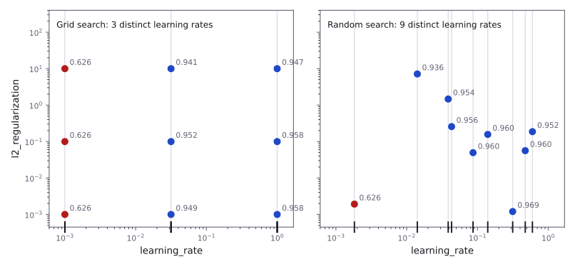
Repeated with 20 different random draws, the random search beat the grid's 0.958 in 16 cases, matched it in 2 and fell below it in 2. Each difference is close to the noise of cross-validation, but the direction is consistent. Bergstra and Bengio (2012) found that for most data sets only a few hyperparameters really matter, and that different ones matter on different data sets. A grid repeats the same few values of each important hyperparameter, whereas every random trial tests a new value. A grid remains appropriate for a few categorical options, such as the two models compared above.
Successive halving
Grid and random search give every configuration the same effort; successive halving discards poor ones early.
function successive_halving(candidates, r_min, r_max, factor):
    r = r_min                    # resource, e.g. a number of trees
    while len(candidates) > 1 and r <= r_max:
        scores = CV score of each candidate, trained with resource r
        n_keep = ceil(len(candidates) / factor)   # factor is η
        candidates = the n_keep candidates with the best scores
        r = r * factor
    return the best candidate of the last round
In scikit-learn, HalvingGridSearchCV and HalvingRandomSearchCV implement it. Both are experimental: they must be enabled by an extra import, and their interface may change without a deprecation period. The example tunes a random forest on the Digits dataset, 1,797 images of handwritten digits of 8 × 8 pixels, with the number of trees as the resource.
from scipy.stats import randint, uniform
from sklearn.datasets import load_digits
from sklearn.ensemble import RandomForestClassifier
from sklearn.experimental import enable_halving_search_cv  # noqa: F401
from sklearn.model_selection import HalvingRandomSearchCV

Xd, yd = load_digits(return_X_y=True)
Xd_train, Xd_test, yd_train, yd_test = train_test_split(
    Xd, yd, test_size=0.2, stratify=yd, random_state=0
)
space = {
    "max_features": uniform(0.05, 0.95),  # from 0.05 to 1.0
    "min_samples_leaf": randint(1, 20),   # from 1 to 19
}
full = RandomizedSearchCV(
    RandomForestClassifier(n_estimators=243, random_state=0),
    space, n_iter=27, cv=5, random_state=0, n_jobs=-1)
full.fit(Xd_train, yd_train)

halving = HalvingRandomSearchCV(
    RandomForestClassifier(random_state=0), space,
    n_candidates=27, factor=3, resource="n_estimators",
    min_resources=9, max_resources=243,
    cv=5, random_state=0, n_jobs=-1)
halving.fit(Xd_train, yd_train)

print(halving.n_candidates_)  # [27, 9, 3, 1]
print(halving.n_resources_)   # [9, 27, 81, 243]
for s in (full, halving):
    print(s.best_params_["max_features"].round(3),
          s.best_params_["min_samples_leaf"], round(s.best_score_, 3))
# 0.186 1 0.97
# 0.186 1 0.97
With the same random_state, both searches draw the same 27 configurations. The full search fits each of them with 243 trees on each of 5 folds: 135 fits and 32,805 trees. Successive halving runs four rounds, of 27, 9, 3 and 1 configurations with 9, 27, 81 and 243 trees. It performs more fits, , but every round grows only 243 trees per fold, trees in all, 15% of the full search. Both searches select the same configuration, and successive halving finishes about seven times faster.
With the default resource, resource="n_samples", the same search used 100, 300 and 900 training samples in three rounds and selected the same configuration. When the resource is a hyperparameter such as n_estimators, max_resources must be set explicitly. The method assumes that a configuration's rank with a small resource predicts its rank with the full resource, so a configuration that needs many samples or trees to perform well can be eliminated early.
Tuning under a time limit
A search multiplies the cost of training by the number of fits, whereas a graded notebook must finish within the task's time limit. At IOAI 2026 the default limit is 20 minutes per notebook, and statements often set less: in Find the Order, 10 minutes cover any training at grading time together with inference.
import time

small_grid = {"max_features": [0.1, 0.3, "sqrt"],
              "min_samples_leaf": [1, 3]}
for n_jobs in [None, -1]:
    search = GridSearchCV(RandomForestClassifier(random_state=0),
                          small_grid, cv=5, n_jobs=n_jobs)
    start = time.perf_counter()
    search.fit(Xd_train, yd_train)
    print(n_jobs, f"{time.perf_counter() - start:.1f} s")

res = pd.DataFrame(search.cv_results_)
print(res["mean_fit_time"].round(2).tolist())  # seconds per fold
print(search.best_params_)
# {'max_features': 'sqrt', 'min_samples_leaf': 1}

# The submitted notebook fits only the chosen configuration
final = RandomForestClassifier(max_features="sqrt",
                               min_samples_leaf=1, random_state=0)
final.fit(Xd_train, yd_train)- Parallel fits.
n_jobs=-1runs the fits on all CPU cores, which makes the search above more than four times faster than on a single core. - Estimated cost. The
mean_fit_timeof a small search predicts the cost of a larger one. - Subsamples. A search on part of the training data is faster but noisier. On 431 of the 1,437 training images, the grid above selects
max_features="sqrt"withmin_samples_leaf=3, the configuration ranked last on the full training set. A subsample is suitable for discarding clearly poor regions, not for the final choice. - Fixed values. The search belongs in development. The submitted notebook contains only the chosen values, as in the last lines of the code.
- Seeds. The
random_stateof a random search fixes the configurations drawn; the estimator and any shuffled splitter need their own. Approaching a Typical Problem covers reproducibility and runtime checks.
The optimism of the best score
best_score_ is the largest of many cross-validated scores, each a noisy estimate of a configuration's performance on new data. Taking the maximum favours estimates that happened to be high, so best_score_ is biased upwards, and the bias grows with the number of configurations compared. In the experiment below the labels are random, so no model can predict new labels better than chance (accuracy 0.5).
rng = np.random.default_rng(0)
X_noise = rng.normal(size=(200, 10))      # random features
y_noise = rng.integers(0, 2, size=200)    # random labels
X_new = rng.normal(size=(10_000, 10))     # new data, same source
y_new = rng.integers(0, 2, size=10_000)

search = GridSearchCV(
    KNeighborsClassifier(),
    {"n_neighbors": range(1, 51), "weights": ["uniform", "distance"]},
    cv=5,
)
search.fit(X_noise, y_noise)
scores = search.cv_results_["mean_test_score"]
print(len(scores), round(scores.mean(), 3))  # 100 0.501
print(round(search.best_score_, 3))          # 0.56
print(round(search.score(X_new, y_new), 3))  # 0.51
The 100 configurations average 0.501, but the best reaches 0.56 by chance, and the selected model scores 0.51 on new data. Over 20 generated datasets, best_score_ averaged 0.576 and the score on new data 0.503. On a single split the gap can have either sign: in the grid search above, the test score of 0.976 exceeds best_score_ of 0.965.
A trustworthy estimate therefore needs data that played no part in the selection: a test set scored once after the search, or nested cross-validation. Repeated submissions to one leaderboard select in the same way, as described in Underfitting and Overfitting.
Resources
| Source | Title | Why read it |
|---|---|---|
| scikit-learn | User Guide: Tuning the hyper-parameters of an estimator | “Exhaustive Grid Search”, “Randomized Parameter Optimization” and “Searching for optimal parameters with successive halving” cover the three search classes used in this module; “Tips for parameter search” covers metrics, pipelines and parallelism. |
| scikit-learn | API: RandomizedSearchCV | Every parameter of the random search, including how lists and SciPy distributions are sampled. |
| scikit-learn | Example: Successive Halving Iterations | Plots how the candidates and resources change from one halving iteration to the next. |
| Bergstra and Bengio, JMLR 13 (2012) | Random Search for Hyper-Parameter Optimization | The paper that argues for random search over grid search when only a few hyperparameters matter. |
| IOAI | 2026 Contest Rules and Technical Appendix | Section 2 lists the available Python libraries, and section 6 gives the default notebook runtime limit. |